links are more likely if the entities are close in latent space. Recent ..... image control localneuron rate test patterns matrix optimal signal gaussian visual size.
A Latent Space Approach to Dynamic Embedding of Co-occurrence Data
Purnamrita Sarkar Machine Learning Department Carnegie Mellon University Pittsburgh, PA 15213
Sajid M. Siddiqi Robotics Institute Carnegie Mellon University Pittsburgh, PA 15213
Abstract We consider dynamic co-occurrence data, such as author-word links in papers published in successive years of the same conference. For static co-occurrence data, researchers often seek an embedding of the entities (authors and words) into a lowdimensional Euclidean space. We generalize a recent static co-occurrence model, the CODE model of Globerson et al. (2004), to the dynamic setting: we seek coordinates for each entity at each time step. The coordinates can change with time to explain new observations, but since large changes are improbable, we can exploit data at previous and subsequent steps to find a better explanation for current observations. To make inference tractable, we show how to approximate our observation model with a Gaussian distribution, allowing the use of a Kalman filter for tractable inference. The result is the first algorithm for dynamic embedding of co-occurrence data which provides distributional information for its coordinate estimates. We demonstrate our model both on synthetic data and on author-word data from the NIPS corpus, showing that it produces intuitively reasonable embeddings. We also provide evidence for the usefulness of our model by its performance on an authorprediction task.
1
Introduction
Suppose we have a graph whose nodes represent entities and whose links represent associations. It is common to ask how we can embed such a graph in a lowdimensional Euclidean space so that nodes which share links tend to be close to one another. Graphs like this often arise when analyzing social networks, distribu-
Geoffrey J. Gordon Machine Learning Department Carnegie Mellon University Pittsburgh, PA 15213
tions of document topics, co-authorship patterns, or recommender systems; the resulting embeddings are useful for tasks like clustering, visualization, information retrieval, and exploratory data analysis. Well-known algorithms for the embedding problem include MDS (Borg & Groenen, 1997), IsoMap (Tenenbaum et al., 2000), Locally Linear Embedding (LLE) (Roweis & Saul, 2000) and spectral clustering (Ng et al., 2001). (Raftery et al., 2002) introduced a model similar to MDS in which entities are associated with locations in p-dimensional space, and links are more likely if the entities are close in latent space. Recent work (Globerson et al., 2004) proposes a novel technique for embedding heterogeneous entities such as author-names and paper keywords into a single space based on co-occurrence counts. Now suppose that, instead of a single graph, we observe a series of graphs which evolve over time, such as co-authorship links for successive years of the same conference. We could embed each year’s graph separately and attempt to align the embeddings from successive years to analyze trends. However, there is no reason to suppose that embeddings from different years would be consistent with one another. Furthermore, we might have limited data for each year, in which case we would expect to find a better embedding for each year by taking into account information from neighboring years. In the limit we might have only a few data points at each time step (for example, imagine coauthorship data from a journal which publishes only a few articles in an issue), and embedding just a single time step’s graph would yield very poor results. In this paper, we extend Globerson et al.’s CODE algorithm to handle time series data. The result is DCODE, a model for dynamic co-occurrence data which provides full distributional information about the embedding coordinates. We show how to approximate the observation model in D-CODE with a Gaussian distribution, so that we can use a Kalman filter to infer coordinates efficiently. The validity of our approxima-
Symbol pa (i), pi pw (j), pj p(ai , wj ), pij A, W, T Φt (A) Ψt (W ) Ct ξi ζj η, Λ µ, Σ ηt|t−1
Definition Marginal empirical prob. of author i Marginal empirical prob. of word j Joint emp. prob. of author i, word j Number of authors,words,timesteps All author coordinates at t All word coordinates at t Co-occurrence counts matrix at t Author coordinate of Taylor expansion Word coordinate of Taylor expansion Canonical parameters of a Gaussian Moment parameters of a Gaussian ηt conditioned on C1 . . . Ct−1
tion is demonstrated experimentally by showing that the resulting embeddings are qualitatively sensible and that they outperform sensible baseline models on a prediction task. While some authors, e.g. Sarkar and Moore (2005), have previously considered time-series co-occurrence data, D-CODE is to our knowledge the first dynamic embedding algorithm which provides principled uncertainty estimates for its coordinates. We present experiments which demonstrate that D-CODE finds highquality embeddings as well as that D-CODE’s uncertainty estimates allow more accurate answers to questions such as the most likely author for a given paper. We also compare our algorithm’s performance with the most natural alternative statistical algorithm, namely PCA over overlapping windows of data, described in more detail in the Experiments section.
2
Φ(A1)
Table 1: Notation
Preliminaries
Our aim is to model the cross-interactions of two sets N of entities over time, denoted by {ai }M i=1 and {wj }j=1 respectively. Data is given to us as a sequence of cooccurrence-count matrices {Ct }Tt=1 , where T denotes the number of discrete timesteps. Thus Ct (i, j) denotes the number of times entity ai interacted with entity wj at time t. In much of this paper, our entity sets are assumed to consist of authors {ai } and words {wj }, and Ct (i, j) denotes the number of times word wj was used by author ai in papers published in year t. For any particular timestep t, we can normalize the counts matrix to obtain joint and marginal empirical probabilities, denoted by pt (ai , wj ) and pt (ai ), pt (wj ). We will drop the subscript t from these probabilities since it will be clear from the context. As in other embedding scenarios, we assume that entity-pair interactions in the data can be explained by real-valued latent variables residing in a lowdimensional space Rk . Let φi and ψj denote the latent random variables corresponding to author ai and word wj respectively. By Φt and Ψt we represent all author
c11
Φ(A2)
φ(a2)
φ(a1)
c12
c21
...
Ψ(W1)
Ψ(W2)
Ψ(Wt)
C1
C2
Ct
c22 ψ(w2)
ψ(w1)
Φ(At)
...
(A)
(B)
Figure 1: Shaded nodes indicate hidden random variables. (A) The graphical model relating author/keyword positions to co-occurrence counts at a single timestep. (B) The corresponding factored statespace model for temporal inference. and word coordinates at time t. We would like to be able to say that pairs of entities closer together in Rk will interact more often. In particular, we will model the count Ct (i, j) as being inversely proportional to the exponentiated squared distance dij = ||φi − ψj ||2 between the latent variables of author ai and word wj . We would like our embeddings to exhibit temporal consistency as well, i.e. coordinates at time t should reflect evidence {C1 , . . . , Ct } accumulated until that time, and not just the data seen at time t. When talking about multivariate Gaussians, we use both the well-known moment parameters (µ, Σ), i.e. the mean and covariance matrix, and the canonical parameters (η, Λ), where Λ = Σ−1 is the precision matrix and η = Σ−1 µ. Additionally, the notation ηt|t−1 denotes the value of a parameter η at time t conditioned on observations from timesteps 1 to t − 1. Table 1 contains the most commonly used notation.
3 3.1
The Algorithm The Single-Timestep Model
As in the CODE model, our basic building block is the probability of a single pairwise author-word interaction given the respective coordinates φi , ψj : p(ai , wj |φi , ψj ) = Z1 p¯(ai )¯ p(wj )e−||φi −ψj || P P 2 Z = ai wj p¯(ai )¯ p(wj )e−||φi −ψj ||
2
(1)
This represents the single-timestep graphical model shown in Figure 1(A). For an entire counts matrix at timestep t, we get the following likelihood (up to a constant depending on the total number of interactions): logP p(CP t |Φt , Ψt ) ∝ − ai wj p¯(ai , wj )||φt,i − ψt,j ||2 − log Z
(2)
CODE obtains point estimates for φ and ψ via gradient descent. Since we treat these latent variables probabilistically but would also like to be computationally
efficient, we choose to model the distribution over entity coordinates at time t, i.e. P (Φt , Ψt | C1:t−1 ), as a Gaussian distribution.
initial estimate of the covariance matrix to reflect a high degree of uncertainty, in order to allow the embedding to adapt to the initial observations.
However, even if we instantiate this joint distribution and initialize it with reasonable values, we cannot obtain a closed form update for P (Φt+1 , Ψt+1 | C1:t ) at the next timestep since the observation likelihood (2) is not Gaussian. So, we will approximate the true observation model by a Gaussian as well, in Section 3.2.1.
3.2.1
3.2
Extension to Dynamic Embedding
The natural choice for our dynamic model is a Kalman Filter (Kalman, 1960), as shown in Figure 1(B). The three standard steps of conditioning (factoring in a new observation to the current belief state), prediction (propagating the belief through the transition model) and rollup (marginalizing to obtain the new belief state) are all closed-form updates assuming that the observation and transition models are Gaussian:
& Rollup: P (Φt+1 , Ψt+1 |C1:t ) = R RPrediction P (Φ t+1 , Ψt+1 |Φt , Ψt )P (Φt , Ψt |C1:t )∂Φt ∂Ψt Φt Ψt (3) The conditioning step decreases uncertainty in the system, and the prediction step increases uncertainty. The conditioning step corresponds a simple addition of corresponding canonical parameters. The resulting Gaussian is characterized by: Φt , Ψt |C1:t ∼ N (ηt|t , Λt|t ) (4)
where (ηobs , Λobs ) are canonical parameters of the observation model. Let us now examine the prediction step. Our transition model is a zero-mean symmetric increase in uncertainty by adding a diagonal noise term, in order to inject uncertainty without biasing the coordinates in any particular direction: Φt+1 , Ψt+1 |C1:t ∼ N (µt+1|t , Σt+1|t ) µt+1|t = µt|t Σt+1|t = Σt|t + Σtransition
In order to obtain a tractable Kalman Filter, we approximate the observation model (2) by a joint Gaussian over all entity positions. However, we are unable to obtain a closed-form solution due to the log-normalization constant log Z. We address this problem by approximating log Z by Taylor expansions around suitably chosen points. This leads to closedform Gaussian parameters as a solution, which is our desired approximate observation model. Though this is an approximation without guarantees, we will show that the resulting models (a) sensibly represent uncertainty in entity coordinates, and (b) outperform alternative models in an author prediction task, indicating the validity of the approximation. Some details are in the Appendix. First-order Taylor approximation of log Z around z gives
Conditioning: P (Φt , Ψt |C1:t−1 , Ct = ct ) ∝ P (Ct = ct |Φt , Ψt )P (Φt , Ψt |C1:t−1 )
ηt|t = ηt|t−1 + ηobs Λt|t = Λt|t−1 + Λobs
Approximate Conditioning Step
(5)
This step controls the degree of diffusion in author and word positions between consecutive timesteps. The Σtransition parameter balances the tradeoff between temporal consistency and the effect of new evidence. For the first timestep, we initialize all coordinates around the origin with some perturbation. We set the
log Z ≈ λZ − 1 − log λ
(6)
where λ = 1/z, and z is the value of Z at φi = ξi , ψj = ζj ∀ i, j. However, direct maximization of the loglikelihood is still difficult since the normalization constant is a sum of exponentiated terms. Therefore, we do a second order Taylor expansion of the exponenT tiated distance term g([φi ψj ]) = e−(φi −ψj ) (φi −ψj ) around ξi , ζj ∀ i, j. We set the ξ, ζ values to µt|t−1 , the predicted conditional means based on the previous timesteps. We found this to be most effective, and this also makes sense since µt|t−1 is the most likely value in the absence of any information. The second-order Taylor approximation of g(x) is: 1 g(x) = g(0) + xT ∇(ξi , ζj ) + xT H(ξi , ζj )x 2
(7)
where ∇(ξi , ζj ) and H(ξi , ζj ) are the gradient and Hessian of g(x) respectively, evaluated at ξi , ζj . They are defined as follows: ∂g )ξi ,ζj = −2e−(ξi −ζj ) ∇1 (ξi , ζj ) = ( ∂φ i
∇2 (ξi , ζj ) =
∂g ( ∂ψ )ξi ,ζj j
T
(ξi −ζj )
(φi − ψj )
= −∇1 (ξi , ζj ) (8)
H=
∂2g T T ∂Φ t 2∂Φt ∂ g ∂ΦT t ∂Ψt
∂2g ∂ΨT t ∂Φt ∂2g T ∂ΨT t ∂Ψt
= ξi ,ζj
µ
H11 H21
H12 H22
(A)
(B)
Figure 2: Two pairs of contour plots of an author’s true posterior conditional (left panel) in a 3-author, 5-word embedding and the corresponding approximate Gaussian posterior conditional obtained (right panel). B is a difficult-to-approximate bimodal case, C is an easier unimodal case.
H11 = 2e−(ξi −ζj )
T
(ξi −ζj )
(2(ξi − ζj )(ξi − ζj )T − I)
T H12 = −H11 , H21 = −H11 , H22 = H22
(9) A few more terms are required for our main result. ˜ to be a symmetric matrix of size k(A + W ) × Define Λ k(A + W ), as in (10). I is the k × k identity matrix, where k is the embedding dimension. In our experi˜ b) denote the 2 × 2 block ments we use k = 2. Let Λ(a, ˜ Λ([2a − 1, 2a], [2b − 1, 2b]). ˜ i) = P pij I2×2 Λ(i, j ˜ + j, A + j) = P pij I2×2 (10) Λ(A i ˜ Λ(i, A + j) = −2pij I2×2 where i ∈ 1 : A, j ∈ 1 : W . All other entries are zero. Define η to be a vector of length k(A+W ) and Λ to be a symmetric matrix of size k(A + W ) × k(A + W ), as in (11) and (12). Let η(a) denote the 2 × 1 sub-vector η([2a − 1, 2a]). P η(i) = pi j pj ∇1 (ξi , ζj ) P (11) η(A + j) = pj i pi ∇2 (ξi , ζj ) ˜ above, we define Using the same notation as Λ P Λ(i, i) = pi j pj H11 (ξi , ζj ) P Λ(A + j, A + j) = pj i pi H22 (ξi , ζj ) Λ(i, A + j) = pi pj H12 (ξi , ζj )
Thus the Gaussian approximation to our observation model has canonical parameters (ηapprox , Λapprox ). In the conditioning step we use (4) to get (ηt|t , Λt|t ). From these, we compute the moment parameters (µt|t , Σt|t ). Now in the prediction and roll-up step we use these parameters to obtain estimates of (µt+1|t , Σt+1|t ) using (5). The resulting Λ may have negative eigenvalues. To project to the closest possible symmetric-positivedefinite matrix, we set the negative eigenvalues to a small positive number. Together these approximations give us a tractable expression while retaining the highly informative inter-coordinate interactions (e.g. x − y correlation in two dimensions). In Figure 2 we compare contour-plots of the true posterior conditional to the one obtained by our method. The true posterior may be multimodal, as in the left panel of Figure 2(A), when it is difficult to approximate with any unimodal distribution. Even then, the corresponding Gaussian is centered reasonably between the two peaks (Figure 2(A) right panel). In most cases we observed, however, the true posterior is unimodal and the approximation is a good fit, though with higher variance (Figure 2(B)).
4 (12)
Let Θt denote the stacked vector [ΦTt ΨTt ]T of all author and word coordinates at time t. The resultant approximate log-likelihood has the following form:
Experiments
We evaluate D-CODE based on the quality of visualizations produced, their temporal consistency and correspondence to the data. We empirically evaluate the usefulness of distributions provided by D-CODE, and see whether useful properties of the distribution are preserved. We also quantitatively test performance on an author-prediction task.
1 ˜ + λΛ)Θ) log p(Ct |Φt , Ψt ) ∝ −C + (−λη T Θ) − (ΘT (2Λ 2 4.1 Algorithms and Tasks Note that it corresponds to a Gaussian in canonical D-CODE The filtering distribution over entity coorform. The final set of observation model parameters dinates learned from dynamic co-occurrence data per thus obtained are: timestep can be used to calculate expected probabilities for prediction. These can be estimated in closed ηapprox = −λη (13) ˜ + λΛ) form using our approximation for log Z, by marginalizΛapprox = (2Λ
5.5 5
Y2
X2
Y1
A2
X1
A3 A2 A1
A3 A1
Y3 X3
A2 A1 A3
X2
X3
Y3 Y2 Y1
Y3 Y1 Y2
X3 X2 X1
4.5 avg rank of X’s given A’s
X1
4 3.5 3 2.5 2
0
(A)
(B)
(C)
Rank w/ expected model probs Rankt w/ MLE estimates only
1.5 10
20
30
40
50
60
(D)
Figure 3: Dynamic embedding of a noisy synthetic data sequence with authors X1 . . . X3 ,Y1 . . . Y3 and words A1 . . . A3 , with 0.95 confidence ellipses. A. Initially the X − A pairs have high co-occurrence counts. B. over time this trend shifts to equal counts, C. and eventually shifts to high co-occurrence counts between Y − A pairs. D. For the same sequence, average predicted rank of authors Xi given words A over time as ranked by Naive Bayes with and without the distributions. Notice the gradual change in D-CODE’s prediction compared to the sharp change when not modeling uncertainty. ing over the latent positions. This is the most powerful model among the alternatives considered, capturing both uncertainty in entity coordinates as well as temporal dynamics. To evaluate the usefulness of dynamic modeling, Static D-CODE is a variant that learns an embedding based on CT −1 to predict coordinates for year T . The alternative of based on embedPprediction T −1 ding the aggregate data t=1 Ct fares worse. D-CODE MLE To evaluate the usefulness of modeling uncertainty in entity coordinates, we can evaluate model probabilities using (1) at µt|t , which is the posterior mean of Φ and Ψ. Static D-CODE MLE is a variant analogous to Static D-CODE described above. Dynamic PCA We compare D-CODE against a dynamic embedding algorithm based on PCA (M.W. Berry & Letsche, 1995) of overlapping windows of the data. We create a new data set by averaging our co-occurrence counts over fixed-size windows of consecutive timesteps to maintain temporal consistency. On the NIPS data we use a window of size 4, heuristically chosen for good performance. For an aggregated counts matrix C over a window, we compute D, which is a diagonal matrix with D(i) = P C(i, j). Let M = ǫI + (1 − ǫ)D−1 C. This dej fines the transition probabilities of a random walk on a graph with words and authors as nodes, and links with respective co-occurrence counts as weights. ǫ is the probability with which at any step the random walk stays at the same node. M p then denotes the transition probabilities of a p-step random walk. Since M is un-symmetric, the standard practice is to work with a symmetric matrix, i.e. N = D1/2 M D−1/2 = ǫI + (1 − ǫ)D−1/2 CD−1/2 . Note that N p = D1/2 M p D−1/2 . The top eigenvector of N is a constant vector. The top k (excluding the first) eigenvectors of N , scaled by eigenvalues raised to powers
of k/2, give us the PCA projection of the counts matrix. We manually picked the ǫ and p for which the algorithm seems to perform best. The projection in the current timestep is transformed via the Procrustes transform (Sibson, 1979) to best align with the previous timestep’s configuration. LLE We embed co-occurrence data using Locally Linear Embedding (Roweis & Saul, 2000). Like the static D-CODE variants above, we embed data for year T − 1 and predict for year T . Since LLE cannot meaningfully embed heterogenous sets of entities based on pairwise counts alone, we define author-author distances based on the words they use, as in Mei and Shelton (2006). This allows us to compare with LLE, though the resulting algorithm sometimes returns degenerate embeddings. We report results from cases with non-degenerate embeddings. Any of the above embedding techniques can then be used to get point estimates of the coordinates, or distribution over the coordinates, using which we perform the following prediction task: Naive Bayes Author Prediction We use the distributions over entity locations at each timestep to perform Naive Bayes ranking of authors given a subset of words from a paper in the next timestep. 4.2
Data sets
NIPS We looked at word-author co-occurrence data over 13 years from the NIPS proceedings of 198619991 . We implemented D-CODE on a subset of the data with the 40 most prolific authors and 428 most common words appearing in their papers. 1
http://www.cs.toronto.edu/ ∼ roweis/data.html
Synthetic We generate a synthetic data set to closely examine D-CODE’s ability to model temporal patterns and represent correlations in its posterior distributions. The data consists of a sequence of co-occurrence counts matrices involving two groups of authors X1 . . . X3 and Y1 . . . Y3 , and a single group of words A1 . . . A3 . The data exhibits three distinct epochs. X − A co-occurrences are high and Y − A are low in the first few timesteps. Afterwards, these cooccurrences start changing slowly until X − A counts are low and Y − A counts are high. 4.3
Visualizing trends and uncertainty in synthetic data
To investigate whether distributions over entity coordinates give us any advantage, we ran D-CODE on the synthetic data set described earlier. Figure 3 illustrates the D-CODE embedding of this data in timesteps from these three distinct periods, along with 95% confidence ellipses of the conditional posterior for each entity, fixing every one else’s locations fixed at their posterior means. The orientation of ellipses around entities is informative. For example, figure 3(A) indicates that uncertainty in Xi locations is most acceptable in directions orthogonal to the A − X axis. This indicates that our variational approximation of the observation model manages to represent uncertainty consistently with the data. We calculated the average rank of authors Xi given the word list A1 , A2 , A3 , A4 over all timesteps using the Naive Bayes prediction. We expect this rank to be close to 2 in the beginning (mean of 1, 2, 3), and drop gradually to 5 to reflect the dynamic trend in the data. The change happens very smoothly over time-steps 20 − 60. Figure 3(D) shows that the ranks induced by D-CODE fulfill this expectation, since ranks change smoothly from low to high over this period. This is because of the increase in uncertainly in author positions, which is also reflected in the enlarged confidence intervals of the X’s in figure 3(B). The MLE estimate, on the other hand is overconfident and switches too abruptly. 4.4
Visualizing the NIPS data
We embedded the NIPS data using D-CODE. The words in different parts of it define different areas of machine learning. We also find the corresponding authors in those areas. For example in figure 4(A) we have presented the embedding of 40 authors and 428 words. These are the overall most popular authors, and the words they tend to use. We can divide the area in the figure in four clear areas, within the rectangles. The top-right region magnified in Figure 4(C) has words like reinforcement,agent,actor,policy,acquisition
authors such as Singh, Dayan and Barto which clearly are words from the field of reinforcement learning. In the top-left region are words like kernel,regularization,error,bound. The other two regions also have noticeable patterns. 4.5
Predicting authors of NIPS papers
We define a prediction task by attempting to rank authors given a set of words, say from a paper taken from a subsequent timestep. D-CODE and D-CODE MLE can calculate the required marginal probabilities p(w | a) for Naive Bayes as described earlier. We can also compute p(w | a) from Dynamic PCA or LLE embeddings by using entity locations as Φ and Ψ in the model probability equation (1). We first describe a few specific author-keyword pairs and their conditional probability-based rank predictions over time. In Figure 5 we plot the rank of particular authors given particular keywords over time according to Naive Bayes prediction with uniform priors, in comparison to the empirical conditional probabilities. In the bottom panels of Figure 5, (Jordan,variational) and (Smola,kernel) have high empirical probabilities in the later timesteps, corresponding to ranks closer to 1 in the top panel according to D-CODE. The prediction according to Dynamic PCA is less consistent and does not correspond to the data nearly as well. In table 2, we show median predicted rank of true authors of papers using embeddings of different sized sets of authors and words, according to Naive Bayes prediction. Note that this is a harsh metric since a paper may have multiple authors and the metric expects each of them to be ranked as first-author, which is impossible. Here our aim is just to compare with alternative models, not to compare with the state of the art. For each size of data set (a, w), random subsets are obtained from the 100 most prolific authors and their 500 most common words. We perform filtering up to t = 12 on the NIPS data, then predict author ranks for all papers in t = 13 with an author included in the embedding. Average predicted rank is calculated for each true-author by ranking all possible authors given words in the paper, noting the rank of the true author, then averaging this measure over all (trueauthor,paper) pairs. This process is repeated for several embeddings, to counter randomness. We see in the table that D-CODE-based predicted ranks are better in most cases. This can be attributed to D-CODE’s usage of distributions. LLE-based embeddings, as well as the static counterparts of D-CODE and D-CODE MLE, perform poorly in most cases. These algorithms, Static D-CODE and Static D-CODE MLE, embed the counts matrix for t = 12 and use it to predict authors for t = 13 with and without using distributions, re-
1.5
policy
0.9
policy
TishbyN
acquisition trading committee reinforcement rivalry 0.8 critic composite Singh conditioning synergy Moody S binocular Tishby DayanJ actor N P agent Smola stack tags routing A feature Scholkopf hyperparameters 0.7 Bcompetition Graf competitive information sv dominance clustering H Vapnik miller regularization V call priceBarto patterns ocular features rate risk attention Obermayer cells pathway A capacity occupancy theorem K functions optimal return method cortex empirical treeadaptation 593 methods Williams LeCun Denker support orientation function cortical associative Mozerlevel acetylcholine vector C kernels kernel characters performance markov aircraft entropy data J memory decision contrast number set Giles SimardYdelays context M Bower algorithm part parts Pimpulse Henderson 0.6 gridaddress centered space template training system phase Jresponse recognizer cun C opt connection state log development Pougettrees probability map eye error D prototypes spike bound distance linear sequences directional figure lgn node matrix recognition equation search tangent neural variables A pitch domain output brain learning solution parietal means fixed process subspace tdnn size schedules time layer classifier writer model pruning test update population task margin tasks normalization hand obdvisual pulse term character approach Bengio current convolution trajectory Stork basis pca control classifiers chain channel manager net position machine region Y obs networks D component network models match arm initial weak dependent side order rbf distribution Muller weight architecture speech recurrent modes interactions scale density lateral jordan bayesian line digit K adaboost mlp forward weights missing path Jordan gaussian attractor controller code graph direction stimulus weighting experts units unit parameters noise sequence states drift hidden TrespM distributed temperature source firing sharing dynamics 0.5 resolution Guyon ann word text factor signatures V statistics signal evolution faces false mst warping tit equations connections board I sex module words Ghahramani interneurons object Sun mouse rap Z Hinton findings movement neuron Waibel neurons local tresp motion G inverse solutions G repetition disparity visible A segmentation Saad codes query Zemel hme Sejnowski Koch D R signature Morgan velocity em T C image images motor mimic N fitness Violaanna variational growing centers Jackel 0.4 P Lee statistic L Kawato speaker Y retrieval vor M Lippmann synapse R digital filtersteacher voltage Murray documents student cue chip A hit flow 0.3 overcomplete circuit
1
0.5
0
−0.5
−1
A
tags
−1.5
−1
−0.5
0
0.5
1
acquisition trading
1.2 hyperparameters
Scholkopf
committee reinforcement
1.1
rivalry
B
competition information 1 sv dominance clustering 0.9 regularization ocular attention Obermayer K occupancy tree WilliamsC
level
Mozer
M
analog facial −1.5 −2
1.3
stack
Smola
1.4
1.5 −1.6
−1.4
−1.2
(A)
patterns risk pathway
SinghS
critic conditioning
composite synergy Moody J Dayan
binocular actor
P
agent
rate 0.8
routing
feature 0.7 functions cortex GrafH competitive function 0.6 orientation adaptation kernels vector markov rate cortical kernel Vapnik miller data V contrast call numberentropy 0.5 features price Barto A algorithm capacity error set part cells support eye parts bound 0.4 Bower theorem return J −0.2 0 0.2 0.4 −1 −0.8 −0.6
(B)
0.6
0.8
(C)
Figure 4: (A). t = 13 Dynamic embedding of NIPS data (1999). (B),(C). Close-ups of roughly the top two boxes in (A), showing regions dominated by distinct sub-fields. 20 15
a=Jordan,w=variational
15
10
10
5
5
20
20
PCA rank
15
15
1
empirical P(a|w)
5 20 PCA rank
15
5
6
8 timestep 9 10
7
11
12
13
0 4
(A)
PCA rank
10 5 1
empirical P(a|w)
empirical P(a|w)
0.5
0.5
0.5
a=Waibel, w=speech DCODE rank
10
5
5
0 4
15
DCODE rank
10
10
1
20
a=Smola , w=kernel
20
DCODE rank
5
6
7
8
9
10
11
12
13
0 4
5
6
(B)
7
8
9
10
11
12
13
(C)
Figure 5: Average author rank given a word, predicted using D-CODE (above) and Dynamic PCA (middle), and the empirical probabilities p(a | w) on NIPS data (below). t = 13 corresponds to 1999. A. Jordan and variational. B. Smola and kernel. C. Waibel and speech. Note that D-CODE’s predicted rank is close to 1 when p(a | w) is high, and larger otherwise. In contrast, Dynamic PCA’s predicted rank shows no noticeable correlation. Table 2: Median predicted rank of true authors of papers in t = 13 based on embeddings until t = 12. Values statistically indistinguishable from the best in each row are in bold. D-CODE is the best model in most cases, showing the usefulness of having distributions rather than just point estimates. D-CODE and D-CODE MLE also beat their static counterparts, showing the advantage of dynamic modeling. Data size (authors,words) 20a, 188w 30a, 289w 40a, 348w
D-CODE 4.1 8 14.2
D-CODE MLE 7.4 10.5 9.5
Static D-CODE 14.4 9 12.8
Static D-CODE MLE 9.5 12 19
Dynamic PCA 7 9 16.8
LLE 11.8 13 21
spectively. This shows the usefulness of modeling dynamics of the data, since information from prior years accumulates in the filtering distribution and aids in making better predictions.
of dynamic embedding, the resulting model is unique in its probabilistic treatment of the coordinates, modeled as latent variables with posterior distributions rather than the point estimates of previous models.
5
While the approximation applied to yield a tractable observation model is uncontrolled, the visualizations in Sections 4.3 suggest that the model obtained still preserves important correlations in the posterior, and the NIPS author prediction results(Section 4.5) con-
Discussion
We have proposed and demonstrated D-CODE, a model for Euclidean embedding of co-occurrence data over time by formulating the problem as a factored state space model. Aside from this novel formulation
firm that these correlations in the posterior translate into superior performance in realistic scenarios. These results also indicate benefits of modeling the dynamics in the data for prediction purposes, and not just for obtaining smooth temporal visualizations. There are several possibilities for future work. There may be a choice of different approximations for the observation model that lead to dynamic models of different kinds, such as particle filters. A Markov Chain Monte Carlo simulation of the exact observation model would allow us to compare the exact shape of the posterior with our Gaussian approximation. There is also room for improvements in the computational aspects. Increasing the numbers of authors and words, or increasing the number of embedding dimensions, both linearly affect the size of the precision matrix that is inverted in the Kalman filter update steps. However, sparseness properties of this matrix could be explored and utilized for faster filtering.
Acknowledgements We are grateful to Carlos Guestrin for valuable discussions. We also thank the reviewers for their insightful comments.
References Borg, I., & Groenen, P. (1997). Modern multidimensional scaling. Springer-Verlag. Globerson, A., Chechik, G., Pereira, F., & Tishby, N. (2004). Euclidean embedding of co-occurrence data. Proc. NIPS. Kalman, R. E. (1960). A new approach to linear filtering and prediction problems. Transactions of the ASME– Journal of Basic Engineering. Mei, G., & Shelton, C. R. (2006). Visualization of collaborative data. Proc. UAI. M.W. Berry, S. D., & Letsche, T. (1995). Computational methods for intelligent information access. Proceedings of Supercomputing. Ng, A., Jordan, M., & Weiss, Y. (2001). On spectral clustering: Analysis and an algorithm. Raftery, A. E., Handcock, M. S., & Hoff, P. D. (2002). Latent space approaches to social network analysis. J. Amer. Stat. Assoc., 15, 460. Roweis, S. T., & Saul, L. K. (2000). Nonlinear dimensionality reduction by locally linear embedding. Science. Sarkar, P., & Moore, A. (2005). Dynamic social network analysis using latent space models. Proc. Nineteenth Annual Conf. on Neural Info. Proc. Systems (NIPS). Sibson, R. (1979). Studies in the robustness of multidimensional scaling : Perturbational analysis of classical scaling. J. Royal Stat. Soc. B.
Tenenbaum, J., de Silva, V., & Langford, J. C. (2000). A global geometric framework for nonlinear dimensionality reduction. Science.
Appendix In this section we give some details of the derivations. We approximate the log-normalizer of the distribution in order to get a Gaussian observation model. We will now look at the log-likelihood in (2). Let us examine the first part. We ignore t here for simplicity. P P − ai wj p¯(ai , wj )||φi − ψj ||2 P P = − ai wj p¯(ai , wj )(φi − ψj )T (φi − ψj ) (14) ˜ = −ΘT ΛΘ ˜ as in (10). We now linBy moment matching, we get Λ earize the second part of (2), i.e. log Z using a Taylor approximation around Φ and Ψ. We do a first-order Taylor expansion around Z leading to Equation (6). This is followed by a second-order Taylor expansion T of the exponentiated distance term e−(φi −ψj ) (φi −ψj ) around ξi , ζj , resulting in (7). The second-order approximation g([φTi ψjT ]), equation (7), becomes = 1 + φTi ∇1 + ψjT ∇2 + 12 [φTi ψjT ]H(ξi , ζj )[φTi ψjT ]T = 1 + φTi ∇1 + ψjT ∇2 + 12 [φTi H11 φi + ψjT H21 φi + φTi H12 ψj + ψjT H22 ψj ] (15) where H(ξi , ζj ) is the Hessian evaluated at ξi , ζj , (9). Also ∇1 (ξi , ζj ) and ∇2 (ξi , ζj ) are the gradients w.r.t. φi and ψj respectively, also evaluated at ξi , ζj , (8). For convenience, define η to be a vector of length 2(A+W ) and Λ to be a symmetric matrix of size 2(A + W ) × 2(A + W ), as in (11) and (12). By i we denote author i and by j we index word j. Now using (11), (12) and (15), log Z becomes: P T log Z = log ij pi pj e−(φi −ψj ) (φi −ψj ) P P P ≈ C + λ[ i φTi η i + j ψjT η j + 21 ( i φTi Λii φi + P P 2 ij φTi Λij ψj + j ψjT Λjj ψj )] = C + λ(η T Θ) + 21 λ(ΘT ΛΘ)
(16) All terms independent of µ, Σ were combined in the constant term C. Using (14) and (16) we obtain the approximate log-likelihood ˜ − C − λη T Θ − 1 λ(ΘT ΛΘ) log p(Ct |Φt , Ψt ) = −ΘT ΛΘ 2 1 T ˜ T = −C + (−λη Θ) − (Θ (2Λ + λΛ)Θ) 2 which gives us a Gaussian distribution with canonical parameters as in (13).