A learnable representation for syntax using ... - Semantic Scholar

A learnable representation for syntax using residuated lattices Alexander Clark Department of Computer Science Royal Holloway, University of London [email protected]

Abstract. We propose a representation for natural language syntax based on the theory of residuated lattices: in particular on the Galois lattice between contexts and substrings, which we call the syntactic concept lattice. The natural representation derived from this is a richly structured context sensitive formalism that can be learned using a generalisation of distributional learning. In this paper we define the basic algebraic properties of the syntactic concept lattice, together with a representation derived from this lattice and discuss the generative power of the formalism. We establish some basic results which show that these representations, because they are defined language theoretically, can be inferred from information about the set of grammatical strings of the language. We also discuss the relation to other grammatical formalisms notably categorial grammar and context free grammars. We claim that this lattice based formalism is plausibly both learnable from evidence about the grammatical strings of a language and may be powerful enough to represent natural languages, and thus presents a potential solution to the central problem of theoretical linguistics.

1

Introduction

Given arbitrary amounts of information about a language, how can we construct a representation for that language? In formal grammar, we define a class of representations for languages, and a function from these representations into the set of languages. Thus we have the class of Context Free Grammars (CFGs), and for each CFG, G, we have the language L(G). Given a grammar, there is an efficient procedure for determining whether a string w ∈ L(G). However, the inverse problem is hard: given information about the strings that are in some language L, there are no good procedures for finding a context free grammar G such that L = L(G). Deciding what the non-terminals of the grammar should be is hard for linguists to do; it requires tenuous lines of argument from unreliable constituent structure tests, and disputes cannot be resolved easily or empirically. Moreover, the end results are inadequate: no one has ever produced a descriptively adequate generative grammar for any natural language. Even in English, the most well studied language, the “correct” analysis is often unclear. The problem is that the representation is radically under-determined by the evidence. Since there are many possible CF grammars for any CF language, indeed

infinitely many for any infinite language, the task is ill defined without additional constraints, or an “evaluation procedure” in Chomskyan terms. The mechanisation of this process – i.e. the problem of grammatical inference – is thus also extremely hard. Even learning regular grammars (i.e. non-deterministic finite state automata) is hard computationally, even in quite a benign learning model [1]; and therefore learning CFGs, or Tree-adjoining grammars is also hard. In this paper, we show that it is possible to define alternative representations that have very attractive properties from a learning point of view. The key insight is contained in [2]: if the representational primitives of the model are defined language theoretically, then the model will be easy to learn in an unsupervised way. Thus rather than defining a representation (like a CFG), and then defining a map from the representation to the language that it defines, we proceed in the opposite direction. We start by defining a map from the language to the representation. This reduces or eliminates the underdetermination of the representation by the language. Traditional algorithms for the inference of deterministic finite state automata exploit this approach implicitly through the Myhill-Nerode theorem; [2] exploit it explicitly through identifying nonterminals in a context free grammar with congruence classes of the language. However neither of these models are descriptively adequate for natural language syntax. Here, we extend [3], and rather than basing our model on the congruence classes of the language, we base it on the lattice structure of those congruence classes: these form a residuated lattice that we call the syntactic concept lattice. This greatly enlarges the class of languages that can be represented. A remarkable consequence, which hints strongly that this approach is on the right track, is that the natural representation derived from these considerations, is in fact not a context free formalism, but rather includes some non context free, mildly context sensitive languages. In addition it is capable of representing richly structured languages, which require structured non-terminals (i.e. augmented with feature structures) to be compactly represented by a context free grammar. It does not include all CFLs, but the examples of those that it does not are bizarre and do not correspond to phenomena in natural language. The contributions of this paper are: 1. a definition of the syntactic concept lattice; 2. a proof that this is a residuated lattice; 3. the definition of a grammatical formalism based on this, which is very close to the learnable class of contextual binary feature grammars [3]; 4. some basic results that establish that these representations can be learned merely from information about which strings are in the language.

2

Contexts and Syntactic Concepts

Distributional learning [4] broadly conceived is the approach that tries to infer representations based on the “distribution” of strings. Given a finite non-empty alphabet Σ, we use Σ ∗ to refer to the set of all strings and λ to refer to the

empty string. A context is just an ordered pair of strings that we write (l, r) – l and r refer to left and right. We can combine a context (l, r) with a string u with a wrapping operation that we write : so (l, r) u is defined to be lur. We will sometimes write f for a context (l, r). Given a formal language L ⊆ Σ ∗ we can consider a relation between contexts (l, r) ∈ Σ ∗ × Σ ∗ and strings w given by (l, r) ∼L w iff lwr ∈ L. For a given string w we can define the distribution of that string to be the set of all contexts that it can appear in: CL (w) = {(l, r)|lwr ∈ L}, equivalently {f |f w ∈ L}. There is a special context (λ, λ): clearly (λ, λ) ∈ CL (w) iff w ∈ L. There is a natural equivalence relation on strings defined by equality of distribution: u ≡L v iff CL (u) = CL (v); this is called the syntactic congruence. We write [u] for the congruence class of u. A learning algorithm based on this gave rise to the first linguistically interesting learnability result for context free languages [2]: this used the congruence classes to be the non terminals of a context free grammar together with the basic rule schemas [uv] → [u][v] and [a] → a. In terms of the syntactic monoid, if X, Y, Z are elements of the syntactic monoid X → Y Z is a production iff X = Y ◦ Z. Thus the algebraic properties of the monoid define the structure of the grammar directly. We can also define the natural dual equivalence relation for contexts (l, r) ≡L (l0 , r0 ) iff for all w, lwr ∈ L iff l0 wr0 ∈ L, and we write [l, r] for the equivalence class of the context (l, r) under this relation.

3

Concept lattice

It was realised first by [5] that the relation ∼L forms a Galois connection between sets of contexts and sets of strings. Galois lattices have been studied extensively in computer science and data mining under the name of Formal Concept Analysis [6] and these distributional lattices have been used occasionally in NLP for lexical analysis, e.g. [7, 8]. For a modern treatment of Galois lattices and lattice theory in general see [9]. For a given language L we can define two polar maps from sets of strings to sets of contexts and vice versa. Given a set of strings S we can define a set of contexts S 0 to be the set of contexts that appear with every element of S. S 0 = {(l, r) : ∀w ∈ S lwr ∈ L}

(1)

Dually we can define for a set of contexts C the set of strings C 0 that occur with all of the elements of C C 0 = {w : ∀(l, r) ∈ C lwr ∈ L}

(2)

We define a syntactic concept to be an ordered pair of a set of strings S and a set of contexts C, written hS, Ci, such that S 0 = C and C 0 = S. A set of strings (contexts) is closed iff S = S 00 (C = C 00 ). Note that for any sets S 000 = S 0 and C 000 = C 0 . Thus for any set of strings S we can define a concept C(S) = hS 00 , S 0 i, and similarly for any set of contexts C, we can define C(C) = hC 0 , C 00 i.

We can define a partial order on these concepts where: hS1 , C1 i ≤ hS2 , C2 i iff S1 ⊆ S2 . S1 ⊆ S2 iff C1 ⊇ C2 . We can see that C(L) = C({(λ, λ)}), and clearly w ∈ L iff C({w}) ≤ C({(λ, λ)}). We will drop some brackets to improve legibility. Definition 1. The concepts of a language L form a complete lattice B(L), called the syntactic concept lattice, where > = C(Σ ∗ ), ⊥ = C(Σ ∗ ×Σ ∗ ), where hSx , Cx i∧ hSy , Cy i is defined as hSx ∩ Sy , (Sx ∩ Sy )0 i and ∨ dually as h(Cx ∩ Cy )0 , Cx ∩ Cy i. It is easy to verify that these operations satisfy the axioms of a lattice. Figure 1 shows the syntactic concept lattice for the regular language L = {(ab)∗ }. Note that though L is infinite, the lattice B(L) is finite and has only 7 concepts. ⊤ = hΣ∗ , ∅i

h[a], [λ, b], i

h[b], [a, λ]i

L = h[ab] ∪ [λ], [λ, λ]i

h[ba] ∪ [λ], [a, b]i

1 = h[λ], [a, b] ∪ [λ, λ]i

⊥ = h∅, Σ∗ × Σ∗ i

Fig. 1. The Hasse diagram for the syntactic concept lattice for the regular language L = {(ab)∗ }. Each concept (node in the diagram) is an ordered pair of a set of strings, and a set of contexts. We write [u] for the equivalence class of the string u, [l, r] for the equivalence class of the context (l, r).

4

Monoid structure

In addition to the lattice structure of B(L), we can also give it a monoid structure. We define the concatenation of two concepts as follows: Definition 2. hSx , Cx i ◦ hSy , Cy i = h(Sx Sy )00 , (Sx Sy )0 i

It is easy to verify that the result is a concept, that this operation is associative, and that 1 = C(λ) is the unit and that this monoid operation respects the partial order of the lattice, in that if X ≤ Y , then W ◦ X ◦ Z ≤ W ◦ Y ◦ Z. This is therefore a lattice-ordered monoid. The left part of Table 1 shows this operation for the language L = {(ab)∗ }. Moreover, we can define two residual operations as follows. We extend the operation to contexts as (l, r) (l0 , r0 ) = (ll0 , r0 r), so (f1 f2 ) w = f1 (f2 w) for two contexts f1 , f2 and a string w. We extend it to sets in the natural way. So for example, C (λ, S) = {(l, yr)|(l, r) ∈ C, y ∈ S}. Definition 3. Suppose X = hSx , Cx i and Y = hSy , Cy i are concepts. Then define the residual X/Y = C(Cx (λ, Sy )) and Y \ X = C(Cx (Sy , λ)) These are unique, and satisfy the following conditions: Lemma 1. Y ≤ X \ Z iff X ◦ Y ≤ Z iff X ≤ Z/Y . Proof. Suppose X ≤ Z/Y ; then Sx0 = Cx ⊇ Cz (λ, Sy ). Therefore (Sx Sy )0 ⊇ Cz , and so (Sx Sy )00 ⊆ Cz0 = Sz , and so X ◦ Y ≤ Z. Conversely suppose that X ◦ Y ≤ Z. Then we know that lxyr ∈ L for any x ∈ Sx , y ∈ SY , (l, r) ∈ Cz . Therefore x must have all of the contexts of the form (l, yr), i.e. Cx ⊃ Cz (λ, Sy ), and so X ≤ Z/Y . Exactly similar arguments hold for X \ Z. Therefore the syntactic concept lattice is a residuated lattice [10]. The map that takes S → hS 00 , S 0 i for arbitrary sets of strings is a 1, ∨, ◦-homomorphism from the “free” residuated lattice of the powerset of Σ ∗ ; but not a homomorphism of ∧. Every language, computable or not, has a unique well defined syntactic concept lattice, which we can use as the basis for a representation that will be accurate for a certain class of languages.

◦ > L 1 R A B ⊥

> > > > > > > ⊥

L > L L > > B ⊥

1 > L 1 R A B ⊥

R > > R R A > ⊥

A > A A > > R ⊥

B > > B B L > ⊥

⊥ ⊥ ⊥ ⊥ ⊥ ⊥ ⊥ ⊥

◦ > AAB A ABB B AB 1 ⊥

> > > > > > > > ⊥

AAB > > > > > > AAB ⊥

A > > > > > > A ⊥

ABB > > AB > > > ABB ⊥

B > AB AB > > ABB B ⊥

AB > > AAB > > > AB ⊥

1 > AAB A ABB B AB 1 ⊥

⊥ ⊥ ⊥ ⊥ ⊥ ⊥ ⊥ ⊥ ⊥

Table 1. The concatenation operation. On the left is the operation for the language L = {(ab)∗ }. R = C(ba), A = C(A) etc. On the right is the concatenation operation for the partial lattice for the context free example described in Figure 2. We write A for C(a) and similarly for AAB, AB, . . . . Note that 1 is an identity, but that this operation is not associative: (A ◦ A) ◦ B 6= A ◦ (A ◦ B). If the result of an operation is > then the operation is vacuous.

5

Partial lattice

The lattice B(L) will be finite iff L is regular. If we wish to find finite representations for non-regular languages we will wish to only model a fraction of this lattice. We can do this by taking a finite set of contexts F ⊂ Σ ∗ × Σ ∗ and constructing a lattice using only these contexts and all strings Σ ∗ . This give us a finite lattice B(L, F ), which will have at most 2|F | elements. We can think of F as being a set of features, where a string w has the feature (context) (l, r) iff lwr ∈ L. Definition 4. For a language L and a set of context F ⊆ Σ ∗ × Σ ∗ , the partial lattice B(L, F ) is the lattice of concepts hS, Ci where C ⊆ F , and where C = S 0 ∩ F , and S = C 0 . For example, consider everyone’s favourite example of a context free language: L = {an bn |n ≥ 0}. The concept lattice for this language is infinite: among other concepts we will have an infinite number of concepts corresponding to ai for each integral value of i. If we take the finite set of the six contexts F = {(λ, λ), (λ, b), (a, λ), (aab, λ), (λ, abb), (λ, ab)}, then we will end up with the finite lattice shown on the left hand side of Figure 2. ⊤=K

⊤ = hΣ∗ , ∅i

h[b] ∪ [abb], {(a, λ)}i

h[b], {(a, λ), (aab, λ)}i

h[ab] ∪ [λ], {(λ, λ)}i

h[λ], {(λ, λ), (λ, ab)}i

h[a] ∪ [aab], {(λ, b)}i

h[a], {(λ, b), (λ, abb)}i

{b, abb}

{b}

h∅, F i

{ab, λ}

{a, aab}

{a}

1 = {λ}

∅

Fig. 2. The Hasse diagram for the partial lattice for L = {an bn |n ≥ 0}, with 6 contexts. The top element > contains all the strings, and the bottom element contains no strings. The empty string λ is below the language concept, as it has the context (λ, ab). On the left we have the true lattice; on the right we have the lattice as inferred from a small set of strings.

We can define a concatenation operation as before hS1 , C1 i ◦ hS2 , C2 i = h((S1 S2 )0 ∩ F )0 , (S1 S2 )0 ∩ F i

This is now however no longer a residuated lattice as the ◦ operation is no longer associative, there may not be an identity element, nor are the residuation operations well defined. The right hand side of Table 1 shows the concatenation operation for the lattice of Figure 2. We lose the nice properties of the residuated lattice, but the concatenation is still monotonic with respect to the lattice order – algebraically this partial lattice is a po-groupoid or lattice-ordered magma. Given this partial lattice, we can define a representation that will map strings to concepts of this lattice. Clearly we have the map w 7→ C(w) where each string is mapped to the correct concept. The concept C(w) is a finite representation of the distribution of the string w, of CL (w). Since there may be infinitely many congruence classes in the language, we cannot hope for this representation to be helpful for all strings, but only for some of the strings. For many strings, the representation we will get will be >, which is vacuous – it tells us nothing about the string. However, what we are interested in is predicting one specific context, (λ, λ), and it may be that we can predict that context exactly. The lattice B(L, F ) will consist of only finitely many concepts, so suppose we have a list of them and that we can compute the operations ∧, ∨, and ◦. Then we can define a recursive function that uses the lattice to compute an estimate of C(w). Definition 5. For any language L and set of contexts F , which therefore defines a lattice B(L, F ), we define φ : Σ ∗ → B(L, F ) recursively by – φ(λ) = C(λ) – φ(a) = C(a) for all a ∈ Σ, (i.e. for all w, |w| = 1) – for all w with |w| > 1, ^

φ(w) =

φ(u) ◦ φ(v)

(3)

u,v∈Σ + :uv=w

or alternatively if we take w = a1 . . . an , φ(w) =

n−1 ^

φ(a1 . . . ai ) ◦ φ(ai+1 . . . an )

(4)

i=1

This is a recursive definition, that can be efficiently computed in O(|w|3 ) time using dynamic programming techniques, analogously to the CKY algorithm. Equation 3 needs some explanation. In B(L), C(u) ◦ C(v) = C(uv). This is not true always in B(L, F ), but we can establish that C(u) ◦ C(v) ≥ C(uv). Thus if w = uv we know that C(w) will be less than C(u) ◦ C(v), and that this will be true for all u, v such that uv = w. Since it is less than all of them, it will be less that the ∧ V over them all since meet is a greatest lower bound. So we know that C(w) ≤ u,v C(u) ◦ C(v). So φ(w) simply recursively computes this upper bound on C(w). In the worst case this will just trivially give >, but we hope that this upper bound will often be tight so that φ(w) = C(w). This may appear to be a slightly circular definition, as it is indeed: however, as we shall see we can

infer the algebraic structure of the lattice in a straightforward way from data, at which point it ceases to be circular. Note that φ(w) aggregates information from every bracketing of w; since ◦ is not in general associative in the partial lattice, each bracketing may give a different result. Moreover, the formalism can combine information from different derivations which is more powerful: this is because W ◦(X ∧Y ) ≤ (W ◦X)∧(W ◦ Y ), but often without equality. This means that it can represent some context sensitive languages, and that the structural descriptions or derivations will no longer be trees, but rather directed acyclic graphs. This map depends on L and F , but we can establish that it is always an upper bound: Lemma 2. For any language L and set of contexts F , for any string w, φ(w) ≥ C(w) This means that the set of contexts predicted will be a subset of the true set of features. Proof. By recursion on length of w, using the fact that C(u) ◦ C(v) ≥ C(uv). Clearly it is true for |w| = 1 and |w| = 0, by construction C(w) = φ(w). Suppose it is true for |w| ≤ k. By definition φ(w) is a meet over the different elements φ(u)◦φ(v), where w = uv. By the inductive hypothesis, φ(u) ≥ C(u), and φ(v) ≥ C(v). Therefore, for each u, v we have that φ(u) ◦ φ(v) ≥ C(u) ◦ C(v) ≥ C(w). C(w) must be less than or equal to the greatest lower bound (meet) of all these φ(u) ◦ φ(v) which is φ(w). Assuming that (λ, λ) ∈ F , we can define the language generated by this representation to be: ˆ = L(B(L, F )) = {w|φ(w) ≤ C((λ, λ))} L

(5)

As a simple corollary we have: Lemma 3. For any language L and for any set of contexts F , L(B(L, F )) ⊆ L. We can define a class of languages L as the set of all languages L such that there is a finite set of contexts F such that L = L(B(L, F )). Since we have made no assumptions at all about L up to now, not even that is is computable, we will find that there are many languages where there is no finite set of contexts that define the language. L is clearly a countable class of recursive languages; we will discuss the language theoretic properties of this class in Section 7, but we will see that it does not correspond to the Chomsky hierarchy. To recap: given the set of contexts F and the language L, we have a uniquely defined partial lattice B(L, F ), that as we shall see can be inferred from data about the language. This lattice can be considered as a representation that computes for every substring an estimate of the distribution of that substring. If this estimate predicts that the substring can occur in the context (λ, λ) then the string is in the language defined by this representation. φ is the recursive computation defined by the lattice that computes this estimate.

6

Learnability

These representations have been defined in language theoretic terms: that is to say, rather than focussing on the function from representation to language, we have focussed on defining a function from the language to the representation. It is therefore straightforward to find learning algorithms for this class. The lattice representation exactly mirrors a fragment of the syntactic concept lattice of the target language. This paper is not focussed on the learning algorithms: see [3] for the first result along these lines. We will state some results that we hope make clear the fundamental tractability of the learning process. First, that if we increase the set of contexts then the language will increase. This, combined with Lemma 3, means that any sufficiently large context set will define the correct language. Lemma 4. If F ⊆ G then L(B(L, F )) ⊆ L(B(L, G)) We will prove this by establishing a more general lemma. We define the obvious map f from B(L, G) → B(L, F ), as hS, Ci 7→ h(C ∩ F )0 , C ∩ F i. and the map back as f ∗ (hS, Ci) = hS, S 0 i. 1 Lemma 5. For any language L, and two sets of contexts F ⊆ G, given the two computational maps φF : Σ ∗ → B(L, F ) and φG : Σ ∗ → B(L, G), then for all w, f (φG (w)) ≤ φF (w). Intuitively this lemma says that when we map from the richer, bigger lattice to the small one, we always get a more specific prediction. Proof. We will use two facts about the map f : f (X ∧ Y ) ≤ f (X) ∧ f (Y ), and f (X ◦ Y ) ≤ f (X) ◦ f (Y ). Again by recursion on the length of w; clearly if |w| = 1, f (φG (w)) = f (C(w)G ) = C(w)F = φF (w). We put a subscript to C()Vto indicate which lattice Inductive step: f (φG (w)) = V we are talking about. V fV( u,v φG (u) ◦ φG (v)) ≤ u,v f (φG (u) ◦ φG (v)) ≤ u,v f (φG (u)) ◦ f (φG (v)) ≤ u,v φF (u) ◦ φF (v) = φF (w). The second lemma is that we can infer B(L, F ) from a finite amount of data. Given a finite set of strings K we can define the lattice B(K, L, F ) in the obvious way: Definition 6. Given a set of strings K and a set of contexts F and a language L, define B(K, L, F ) to be the complete lattice formed by the ordered pairs hS, Ci, where S ⊆ K, C ⊆ F , and where S 0 ∩ F = C, and C 0 ∩ K = S. To avoid problems, let us be clear. The concepts are ordered pairs that consist of a finite set of strings, from K, and a finite set of contexts from F . 1

The two maps f, f ∗ form a residuated pair in that f (X) ≤ Y iff X ≤ f ∗ (Y ), for any X ∈ B(L, G) and Y ∈ B(L, F ).

Definition 7. Let hS1 , C1 i and hS2 , C2 i be in B(K, L, F ). So S1 , S2 are subsets of K. Define a set of contexts (S1 S2 )0 ∩ F . If this set of contexts is closed in B(K, L, F ), then we define the concatenation hS1 , C1 i ◦ hS2 , C2 i = h((S1 S2 )0 ∩ F )0 ∩ K, (S1 S2 )0 ∩ F i. Otherwise it is undefined. Example 1. Suppose L = {(ab)∗ } and F = {(λ, λ), (a, λ), (λ, b), (a, b)}, and K = {λ, a, b}.. B(K, L, F ) will have 5 concepts >, ⊥, C(a), C(b), C(λ). If we try to compute C(a) ◦ C(b), everything is fine. We have ab which has contexts (λ, λ) which is closed, so C(a) ◦ C(b) = C((λ, λ)). But if we try to compute C(b) ◦ C(a), we will get the singleton set of strings {ba}, which has context set {(a, b)} which while it is closed in B(L, F ) is not closed in B(K, L, F ). Definition 8. The lattice B(K, L, F ) is closed under concatenation if for every pair of concepts X, Y , the concatenation X ◦ Y is defined. Note that B(L, F ) is exactly the same as B(Σ ∗ , L, F ). So in order to compute B(K, L, F ) we need to know which strings in F KK are in L; computationally then the algorithm is given F, K and the finite set of strings (F KK) ∩ L. Lemma 6. For any L, F , there is a finite set K such that B(K, L, F ) is closed under concatenation and is isomorphic to the B(L, F ). Proof. (Sketch) For each concept in the finite set of concepts {C(u) ∈ B(L, F )|u ∈ Σ ∗ } pick one such string u. For each pair of concepts X, Y and context f where f is not in X ◦ Y pick a pair of strings u, v such that u ∈ X, v ∈ Y and uv does not have the context f . Moreover as we increase the set of strings K that we are basing the lattice on, the language defined by the lattice will decrease. Intuitively, as we increase the sample size the set of context shared by all samples in a given set will only decrease; thus the predicted set of features will decrease, and φ will move higher in the lattice, thus reducing the language. Definition 9. If J ⊂ K we define the map g from B(J, L, F ) to B(K, L, F ), i.e. from the smaller lattice to the larger lattice as the map that takes hS, Ci to hC 0 ∩ K, Ci, and the map g ∗ from B(K, L, F ) to B(J, L, F ), by hS, Ci 7→ hS ∩ J, (S ∩ J)0 ∩ F i. This is well-defined since S ∩ J will be closed in B(J, L, F ). Lemma 7. For all J, K closed, J ⊂ K, and for all strings w; we have that g(φJ (w)) ≤ φK (w). Proof. (Sketch) Again by induction on length of w. Both J and K include the basic elements of Σ and λ. Suppose true for all w of length at most k, and take some w of length k + 1. We use some inequalities for g that we do not prove

here. φK (w) =

^

φK (u) ◦ φK (v)

u,v

≥

^

g(φJ (u)) ◦ g(φJ (v))

u,v

≥

^

g(φJ (u) ◦ φJ (v))

u,v

! ≥g

^

φJ (u)) ◦ φJ (v))

= g(φJ (w))

u,v

As a corollary we therefore have: Lemma 8. For any L, F and any sets of strings J, K s.t Σ ∪ {λ} ⊆ J ⊆ K and where both B(J, L, F ) and B(K, L, F ) are closed under concatenation, L(B(J, L, F )) ⊇ L(B(K, L, F )) ⊇ L(B(L, F )). Finally we note that there are efficient scalable algorithms for computing these lattices and identifying the frequent concepts; see for example [11]. Thus, for any sufficiently large set of contexts the lattice B(L, F ) will define the right language; there will be a finite set of strings K such that B(K, L, F ) is isomorphic to B(L, F ), and there are algorithms to construct these lattices from K, F and information about ∼L . This is still some way from a formal polynomial learnability result. Since the class of languages is suprafinite, we cannot get a learnability result without using probabilistic assumptions, which takes us out of the scope of this paper, but see the related learnability result using a membership oracle in a non probabilistic paradigm in [3]. Note however that the monotonicity lemmas in the current approach (Lemmas 5 and 7) are exactly the opposite of the monotonicity lemmas in [3]. Space does not permit a full example, but consider the CF language L = {an bn |n ≥ 0}. If F = {(λ, λ), (λ, b), (a, λ), (λ, abb), (aab, λ)}, it is easy to verify that L(B(L, F )) = L. If K = {λ, a, b, ab, aab, abb}, then B(K, L, F ) is isomorphic to B(L, F ). This is shown on the right hand side of Figure 2. Algorithms based on heuristic approximations to this approach are clearly quite feasible: consider sets of contexts of the form (Σ ∗ a, bΣ ∗ ) where a, b ∈ Σ; take all frequent contexts; take all frequent substrings; approximate the relation (l, r) ∼L w probabilistically using a clustering algorithm.

7

Power of the representation

We now look at the language theoretic power of this formalism, and its relationship to other existing formalisms. We will define L to be the class of all languages L such that L(B(L, F )) = L for some finite set of contexts F . The following propositions hold:

– L contains the class of regular languages. – L contains some languages that are not context free. – There are some context free languages that are not in L. The CBFG formalism is clearly closely related. However CBFGs only use the partial order and not the full lattice structure: moreover the absence of unary rules for computing ∧ limits the generative power. Note also the relation to Range Concatenation Grammars [12] and Conjunctive Grammars [13]. 7.1

Categorial grammars

We have shown that this concept lattice is a residuated lattice; the theory of categorial grammars is based largely on the theory of residuation [14]. It is worth considering the relation of the residuation operations in the concept lattice to the theory of categorial grammars. Clearly implication → in categorial grammar corresponds to ≤ in this algebraic framework. Every sequent rule such as X → Y /(X\Y ) can be stated in B(L) as C(X) ≤ C(Y )/(C(X)\C(Y )): an inequality which is true for all residuated lattices. In terms of the sets of axioms, the concept lattice satisfies the axioms of the associative Lambek calculus L. However from a logical point of view the calculus that we use is more powerful. Just as the Ajdukiewicz-Bar-Hillel calculus which only uses the symbols \, / was extended to the associative Lambek calculus with the symbol ◦, here we need to add the additional symbols ∧, ∨ from the lattice operations, together with additional inference rules. Indeed it is the following inference rule that takes us out of the context free languages, since they are not closed under intersection: Γ →Y Γ →Z Γ →Y ∧Z Given that [15] showed that the equational theory of residuated lattices is decidable, this means that the calculus derived from this formalism is also decidable. However the approach taken in this paper is profoundly different: in the categorial grammar style formalism, the underlying model is the residuated lattice of all subsets of Σ ∗ , which is a different lattice to B(L). The language is then defined equationally through the type assignments to the letters of Σ. Here the model is the syntactic concept lattice, and the language is defined algebraically through a direct representation of the algebraic structure of part of the lattice. It is not obvious therefore that the two approaches are potentially equivalent: we can convert the partial lattice into a set of equations, and define the full lattice to be the free residuated lattice generated by Σ and these equations, but it may not be possible to “lexicalise” these equations. 7.2

Context free grammars

We can also consider the relation to context free grammars. Using standard notation, for a CFG, with a non-terminal N we can define the yield of N as ∗

Y (N ) = {w ∈ Σ ∗ |N ⇒ w}

and the distribution as ∗

C(N ) = {(l, r) ∈ Σ ∗ × Σ ∗ |S ⇒ lN r} It is natural to think that hY (N ), C(N )i ∈ B(L(G)). This is sometimes the case but need not be; indeed from a learnability point of view this is the major flaw of CFGs: there is no reason why there should be any simple correspondence between the concepts of the language and the structure of the grammar. There are CFLs for which it is impossible to find CFGs where all of the non-terminals are syntactic concepts, indeed there are some where some of the non-terminals must correspond to concepts with context sensitive sets of strings. However we can represent all CFLs that have context free grammars that have a “Finite Context Property”: Definition 10. For a context free grammar G, a non-terminal N has the FCP iff there is a finite set of contexts F (N ) such that {w|∀(l, r) ∈ F (N ) lwr ∈ L} is equal to Y (N ) If every non-terminal has the FCP, then it can be shown that the partial lattice with the union of all the F (N ), will define the same language as L. This means that for every non-terminal in the grammar, we must be able to pick a finite set of contexts, that suffice to pick out the strings that can be derived from that non-terminal: F (N ) will normally be a subset of C(N ). A single context normally suffices for the simple examples in this paper, but not in natural languages where lexical ambiguity and coordination mean that one may need several contexts to pick out exactly the right set of strings. So for example the context “I was — .”, does not pick out an adjective phrase as “a student” can also appear in that context. 7.3

Context Sensitive

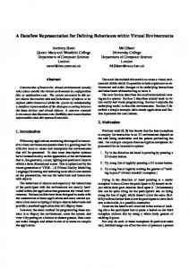
We can also define some non-context free languages. In particular, we define a language closely related to the MIX language (consisting of strings with an equal number of a’s, b’s and c’s in any order) which is known to be non context-free. Example 2. Suppose we have a context sensitive language Let M = {(a, b, c)∗ }, we consider the language L = Labc ∪ Lab ∪ Lac where Lab = {wd|w ∈ M, |w|a = |w|b }, Lac = {we|w ∈ M, |w|a = |w|c }, Labc = {wf |w ∈ M, |w|a = |w|b = |w|c }. It is easy to see that this language is non context free. We define the set of contexts: F = {(λ, λ), (λ, d), (λ, ad), (λ, bd), (λ, e), (λ, ae), (λ, ce), (λ, f ), (ab, λ), (ac, λ)} The resulting lattice is shown in Figure 3. It can be shown that this lattice will define the correct context sensitive language.

Fig. 3. Lattice for the context sensitive example. We will write triples of numbers to refer to subsets of M . So [n, n, n + 1] refers to the set of strings {w ∈ M |∃n, |w|a = n, |w|b = n, |w|c = n + 1}. [n,n,m]d

( ab,)

L

[n,m,n]e

(ac,)

[n+1,n,n]

[n+1,n,n+2]

[n,m,n]

bottom

[n+1,n+1,n]

[n,m,n+1]

[n+1,n+2,n]

[n+1,m,n]

features for [n,m,n]

top

[n,n+1,n+1]

[n+1,n,m]

[n+1,n,n+1]

[n,n+1,m]

features for [n,n,m]

[n,n,n+1]

[n,n,m]

[n,n+1,n]

[n,n,n]

8

Compact Representation

We have defined a representation which is finite, but it is not very compact since the representation may be exponentially large in the number of contexts. In many cases, the number of concepts is polynomially bounded, but it is clearly desirable to use a more efficient representation. Moreover in natural language, we need efficient ways of representing combinations of number, case and gender features in those languages that have them: such features cause an exponential explosion in the number of atomic categories required [16]. The concepts of B(L, F ) are pairs hS, Ci where S is a possibly infinite set of strings and C is a subset of the finite set F . We can thus represent the concepts through the sets C, which are the closed context sets of the lattice: that is to say where C 00 = C. Not all sets of contexts are closed. We will write F (hS, Ci) = C, for the set of contexts of a concept, and F (B(L, F )) for the set of closed context sets. We can therefore represent the concepts as subsets of F , i.e. as bitvectors of length |F |. Looking at Equation 3, we need to be able to perform some computations: the partial order ≤, the meet ∧ and the concatenation operation ◦. Clearly F (X ∧ Y ) will contain F (X) ∪ F (Y ), but it may also contain other contexts, as F (X) ∪ F (Y ) might not be closed. We need to define some efficient scheme for determining which additional elements of F need to be added. For any concept X we can define the set of unordered pairs of concepts H + (X) = {{Y, Z} : Y ∧Z ≤ X}, with the natural partial order. Clearly this is a down set in the sense that if {Y, Z} ∈ H + and W ≤ Y then {W, Z} ∈ H + , so it is natural to represent it through its maximal elements. Let H max (X) be the set of maximal elements of H + (X); clearly one such element will be the vacuous one {X, >}, but there will also be other non-trivial ones: if f ∈ F (X ∧ Y ) \ (F (X) ∪ F (Y )), then {X, Y } ∈ H + (C(f )) but will not be below {C(f ), >}, so there will be a non-trivial element. Given H max (C(f )) for all the features f , we can compute F (X ∧ Y ) efficiently. We can proceed in the same way for concatenation: for a given concept Z define G+ (Z) to be the set of ordered pairs G+ (Z) = {(X, Y )|X ◦ Y ≤ Z}

(6)

This is a set of ordered pairs, not unordered as before, and we can again take the maximal elements Gmax (Z). There will normally be four trivial elements of Gmax (Z) which are (Z, 1) and (1, Z), and (⊥, >), (>, ⊥); not necessarily distinct. As before, it suffices to use only concepts Z which correspond to individual features f : thus we can just store Gmax (C(f )). Space does not permit a full definition of this more compact representation. Looking at this compact representation of the formalism, we can show that it is more expressive than context free grammars. Let Σn be an alphabet of size n; Define Ln = {w ∈ Σn∗ ||w|ai > 0∀i}; i.e. each letter must occur at least once in w. This is an infinite regular language. There is a compact lattice grammar polynomial in n, which defines this language, but an exponentially sized context free grammar would be required to represent it [17].

From a learnability point of view, the compact representation is interesting since the pairs in Gmax and H max are of concepts that are high up in the lattice, and thus consist of large sets of strings – it is clearly easier to learn a small number of larger concepts, than a large number of small concepts.

9

Conclusion

We have presented a model for syntax as an alternative to CFGs and categorial grammars. These models have deep roots in the study of post-Harris structuralist linguistics in Europe; see for example the work surveyed in [18]. We base the representation on an algebraic structure defined by the language: the syntactic concept lattice. Algebraic properties of this lattice can be converted directly into the “grammar”: this largely removes the arbitrariness of the representation, and leads to inference algorithms, as well as consequences for decidability, the existence of canonical forms etc. Given the language, and the set of features, the representation is determined. Selecting the set of features is easy as any sufficiently large set of features will define the same language. If the set of features is too small, then the representation will define a subset of the correct language. One objection to this approach is that it doesn’t produce the “right” results: the structural analyses that we produce do not necessarily agree with the structures that linguists use to describe sentences, for example in treebanks. But of course linguists don’t know what the right structures are: tree structures are not empirical data, but rather theoretical constructs. It is certainly important that the models support semantic interpretation, but as we know from categorial grammar this does not require traditional constituent structure. Moreover, the residuated lattice structure we use has been studied extensively in the model theory for various logics; we therefore conjecture that it is possible to build semantic analysis on this lattice in a very clean way. Ultimately, we don’t yet know what the “right” representations are, but we do know they are learnable. It seems reasonable therefore to start by looking for learnable representations. Just as with context free grammars, we can define a derivation that will “prove” that the string is grammatical. With lattice grammars, rather than being trees, these will be directed acyclic graphs or hypergraphs, where the nodes are associated with a particular span or segment of the input string, and each node is labelled with a concept. Looking at the context sensitive example discussed above, it is clear that the derivation cannot in general be a tree. We think that minimal derivations will be particularly interesting for semantic interpretation: a derivation is minimal if the concept associated with a span cannot be replaced by a more general concept, while still maintaining the validity of the associated DAG. In this case, classical cases of lexical and syntactic ambiguity will give rise to structurally distinct minimal derivations. In general, there will not be a one-to-one map between derivations and semantic interpretations: rather there will be what is called in CG parsing “spurious ambiguity”. If the set of features is large, then the number of possible derivations will increase. For a regular

language, if we have one context out of each context class, we will have structural completeness, and every tree can give rise to a derivation. The other important difference with a CFG is that the labels in the structural descriptions of sentences are not atomic symbols, as is this case with a non-terminal in a CFG, but rather are elements of a lattice. Converting an existing CFG into a lattice grammar is not always possible: however for CFGs that are models for natural languages it should be straightforward. All that is needed is to find a finite set of contexts that picks out the yield of each non-terminal: given a large sample of positive example trees generated by the CFG in question will give a large sample of C(N ) and Y (N ), for any non-terminal N . However this is not the right approach: we are not interesting in representing CFGs, but in representing natural languages, and the limitations of CFG as representations of natural language are very well known. The most radical property of lattice grammars is this: lattice grammars in this approach are not written by human linguists, rather they are determined by the data. The normal activity of linguistics is that some interesting data are discovered and linguists will manually construct some appropriate analysis together with a grammar for the fragment of the language considered. There are normally many possible grammars and analyses. With lattice grammars, the data decides: there is no role for the linguist in deciding what the appropriate structural description for a sentence is. The linguist can decide what the contexts are, and how many are used, and thus can control to some extent the set of possible structural descriptions, but given the set of contexts, the rules and the possible analyses for individual sentences are fixed given agreement about the data. There is an interesting link to the classic presentation found in traditional descriptive grammars, such as [19]. In such grammars, the syntactic properties of a word are described through their occurrences in sample sentences: the lattice approach allows a fairly direct translation of this description into a generative grammar: Consider for example adjectives in English, which typically appear in three positions attributive, predicative, and postpositive, and which accept degree modifiers and adverb modifiers [19, p.528]. Each of these properties can be associated with a context, writing the gap as “—” “They are —”, “I saw some — people” , “There is someone —”, “They are very —”, “He is the most — person I know”, “He was remarkably —”. A word like “happy” can appear in all of the contexts. These lattice based models potentially satisfy the three crucial constraints for a model of language [20]; they may be sufficiently expressive to represent natural languages compactly, they can be learned efficiently, and they do not posit a rich domain specific and evolutionary implausible language faculty. We suggest they are therefore worthy of further study.

References 1. Angluin, D., Kharitonov, M.: When won’t membership queries help? J. Comput. Syst. Sci. 50 (1995) 336–355

2. Clark, A., Eyraud, R.: Polynomial identification in the limit of substitutable context-free languages. Journal of Machine Learning Research 8 (Aug 2007) 1725– 1745 3. Clark, A., Eyraud, R., Habrard, A.: A polynomial algorithm for the inference of context free languages. In: Proceedings of International Colloquium on Grammatical Inference, Springer (September 2008) 29–42 4. Harris, Z.: Distributional structure. In Fodor, J.A., Katz, J.J., eds.: The Structure of Language. Prentice-Hall (1954) 33–49 5. Sestier, A.: Contribution a ` une th´eorie ensembliste des classifications linguistiques. In: Premier Congr`es de l’Association Fran¸caise de Calcul, Grenoble (1960) 293–305 6. Ganter, B., Wille, R.: Formal Concept Analysis: Mathematical Foundations. Springer-Verlag (1997) 7. Popa-Burca, L.: On algebraic distributional analysis of romanian lexical units. In Kay, M., ed.: Abstracts of the 1976 International Conference on Computational Linguistics COLING. (1979) 54 8. Basili, R., Pazienza, M., Vindigni, M.: Corpus-driven unsupervised learning of verb subcategorization frames. Proceedings of the 5th Congress of the Italian Association for Artificial Intelligence (AI* IA97) (1997) 9. Davey, B.A., Priestley, H.A.: Introduction to Lattices and Order. Cambridge University Press (2002) 10. Jipsen, P., Tsinakis, C.: A survey of residuated lattices. Ordered Algebraic Structures (2002) 19–56 11. Choi, V.: Faster algorithms for constructing a galois/concept lattice. In: SIAM Conference on Discrete Mathematics 2006, University of Victoria, Canada (2006) 12. Boullier, P.: Chinese Numbers, MIX, Scrambling, and Range Concatenation Grammars. Proceedings of the 9th Conference of the European Chapter of the Association for Computational Linguistics (EACL 99) (1999) 8–12 13. Okhotin, A.: Conjunctive grammars. Journal of Automata, Languages and Combinatorics 6(4) (2001) 519–535 14. Moortgat, M.: Multimodal linguistic inference. Journal of Logic, Language and Information 5(3) (1996) 349–385 15. Ono, H., Komori, Y.: Logics Without the Contraction Rule. The Journal of Symbolic Logic 50(1) (1985) 169–201 16. Gazdar, G., Klein, E., Pullum, G., Sag, I.: Generalised Phrase Structure Grammar. Basil Blackwell (1985) 17. Asveld, P.: Generating all permutations by context-free grammars in Chomsky normal form. Theoretical Computer Science 354(1) (2006) 118–130 18. Marcus, S.: Algebraic Linguistics; Analytical Models. Academic Press, N. Y. (1967) 19. Huddleston, R., Pullum, G., Bauer, L.: The Cambridge grammar of the English language. Cambridge University Press New York (2002) 20. Jackendoff, R.: Alternative minimalist visions of language. Proceedings of Chicago Linguistics Society (41) (2008)