A Learning-Based Jam Session System that Imitates a Player’s Personality Model Masatoshi Hamanaka1), 2), Masataka Goto3), 2), Hideki Asoh2), and Nobuyuki Otsu2), 4) 1) Research Fellow of the Japan Society for the Promotion of Science, 2) National Institute of Advanced Industrial Science and Technology (AIST), 3)“Information and Human Activity,’’ PRESTO, JST, 4) University of Tokyo Mbox 0604, 1-1-1 Umezono, Tsukuba, Ibaraki 305-8568, Japan
[email protected] Abstract This paper describes a jam session system that enables a human player to interplay with virtual players which can imitate the player personality models of various human players. Previous systems have parameters that allow some alteration in the way virtual players react, but these systems cannot imitate human personalities. Our system can obtain three kinds of player personality models from a MIDI recording of a session in which that player participated – a reaction model, a phrase model, and a groove model. The reaction model is the characteristic way that a player reacts to other players, and it can be statistically learned from the relationship between the MIDI data of music the player listens to and the MIDI data of music improvised by that player. The phrase model is a set of player’s characteristic phrases; it can be acquired through musical segmentation of a MIDI session recording by using Voronoi diagrams on a piano-roll. The groove model is a model that generates onset time deviation; it can be acquired by using a hidden Markov model. Experimental results show that the personality models of any player participating in a guitar trio session can be derived from a MIDI recording of that session.
1 Introduction Our goal is to create a jam session system in which virtual players react as if they were actual human players. We want to make it possible for a human player to interact, whenever they like, with a virtual player that can imitate whoever the human player wishes to perform, for example, with a familiar, professional, or deceased player, or even with themselves. What is most important in imitating players is to acquire the player’s personality models of a target human player. Previous session systems have not been able to imitate a human player’s personality. Some systems [Aono et al., 1995] have been designed to follow the performance of a human soloist, but without considering the individual character of the virtual player. Although JASPER [Wake
et al., 1994] has a set of rules that determine the system’s reactions and VirJa Session [Goto et al., 1996] has parameters for altering how it reacts, these systems cannot develop player personality models of an actual human player. To realistically imitate a human player, a system must be able to acquire player personality models of that player. The imitating virtual player can then improvise according to the models. The Neuro-Musician [Nishijima and Kijima, 1989; Nishijima and Watanabe, 1992] can learn the relationship between 30 sets of an 8-bar-length input pattern and an output pattern by using neural networks. However, it is only capable of dealing with the limited style of a jam session where a solo part must be changed in 8-bar rotation. In other words, a virtual player and a human player cannot both play a solo part in the same time. Moreover, the Neuro-Musician must prepare a training set of 8-bar-length input-output data to enable neural network learning. In an actual jam session, a player does not always play an 8-bar solo to the 8-bar solo of the other players. Therefore, we cannot acquire the player models from a MIDI session recording by using the Neuro-Musician method. On the other hand, the Band-OUT-of-a-Box (BoB), which deals with a problem similar to ours [Thom, 2001a; Thom, 2001b], indicates that machine learning techniques provide a useful approach to acquire a player’s models. However, BoB can only react to a human performance of an immediately previous four bars. It has a fixed relationship in which the human player is the leader and the virtual player is the follower. Our jam system allows us to acquire player personality models of a target human player from the MIDI1 recording of a session in which that player participated. The main advantage of our approach is that we do not have to directly evaluate the target player: all we need to build the models is session recording data.
2 A Guitar Trio Session System Our system deals with constant-tempo 12-bar blues performed by a guitar trio. Figure 1 shows a jam session 1
MIDI stands for Musical Instrument Digital Interface.
past Human
Virtual Imitating
MI D
I
DI MI
Guitar Trio Session Human
Virtual Imitating
MIDI
Virtual Imitating
model in which either a human or the computer can be selected to perform the part of each player. We can imagine sessions in which all players will be human players just as we can imagine sessions in which all players are computer players. The three players take the solo part one after another without a fixed leader-follower relationship. We obtain three kinds of player personality model from a MIDI session recording – a reaction model, a phrase model, and a groove model. The system has two modes, a learning mode and a session mode. In the learning mode (discussed in Sections 3, 4, and 5), the system acquires player personality models in non-real time. These models are stored in a database and different personality models can be assigned to the two virtual players before session play (Figure 2). In the session mode (discussed in Section 6), a human player can interact with the virtual players in real time. Personality database Reaction-model database Phrase-model database Personality model
Groove-model database
Figure 2: Virtual player and personality databases
3
Player A
past performance of A
Player B
past performance of B
Player C
past performance of C
future
next performance of B
Player B's Reaction model
Figurer 3: Player’s reaction model Human
Figurer 1: Session model in which either human or computer can be selected as each player.
Virtual Player
present
Learning a reaction model
A reaction model is the characteristic way that a player reacts to other players. Acquiring an actual player’s individual reaction model is necessary to create a virtual player that reacts as that actual human player does. As shown in Figure 3, each virtual player listens to the performances of all the players (including its own) and uses the reaction model to determine what its next reaction (output performance) will be. The main issue in deriving
the reaction model is to learn the relationship between the input and the output of the target player in MIDI recordings. This can be formulated as a problem of obtaining a mapping from the input to the target player’s output. However the direct MIDI-level learning of this mapping is too difficult because the same MIDI-level sequence rarely occurs more than once and the mapping itself is too sparse. We therefore have introduced two intermediate subjective spaces: an impression space and an intention space (Figure 4). 3.1 Impression space The impression space represents the subjective impression derived from the MIDI input. By applying principal components analysis (PCA) to the results of subjective evaluations of various MIDI performances, we determined three coordinate axes for the impression space. PCA is a statistical method for reducing the number of dimensions while capturing the major variances within a large data set. While listening to a performance, a subject subjectively evaluated it by using ten impression words to rank the performance’s impression on a scale of one to seven. The three selected axes of the impression space represent qualities that can be described as appealing, energetic, and heavy. To obtain a vector in this space, an impression vector corresponding to the MIDI input, we use canonical correlation analysis (CCA). This analysis maximizes the correlation between various low-level features of the MIDI input (such as pitch, note counts, tensions, and pitch bend) and the corresponding subjective evaluation. Since an impression vector is obtained from an individual player’s performance, we have at every moment three impression vectors (Figure 4). The impression space is necessary for learning the relationship between various input performances and the corresponding output performances. If we represent the input performances as short MIDI segments without using the impression space, the same MIDI segments will not be repeated in different sessions. The impression space enables the abstracting of subjective impressions from input MIDI data and those impressions can be repeated. Even if two segments of the input MIDI data differ, they can be represented as a similar vector in the impression space as long as they give the same impression.
input performances of the three players Virtual player B
Virtual player A
impression space
Human player C
low-level features of MIDI data
we determined the three dimensions of this space. Because the number of the short phrases is limited, those phrases are sparsely placed in the intention space. When generating the output, the system selects the output phrase close to the determined intention vector: an appropriate phrase can be selected even if the phrase database does not have a phrase that is exactly placed on the intention vector.
3.3 Player B's reaction model Player A's reaction model
intention space Output performances Figure 4: Player architecture.
Figure 5 shows the transition of the rated values for the impression word “appealing.” The black line represents the value calculated by the system and the gray line represents the value as evaluated by a human listener. For 92 percent of the performance, the calculated and subjectively evaluated values do not differ by more than 1. system subject
7 6 scale
5 4
r2 φ (r ) = exp − 2 σ (k ) r = x − ci
3 2 1
2
4
6
8
10
12
14
16
18
20
22 24[bars]
Figure 5: Transition of rated values calculated by system and evaluated by subject (for impression word “appealing”).
3.2
Acquiring a reaction model
We can regard the mapping from the impression space to the intention space as the reaction model. To derive this mapping function statistically, we obtain various training sets from the target session recordings. These sets are pairs of impression vectors obtained from the three players during a sequence of the past twelve bars and the corresponding next intention vector. For this learning we use Gaussian radial basis function (RBF) networks [Chen et al., 1991]. The RBF networks have one hidden layer with nonlinear inputs, and each node in the hidden layer computes the distance between the input vector and the center of the corresponding radial basis function. The input of the RBF network is impression vector x (L dimensions) derived from three players and the output of the RBF network is intention vector ~y1 , ~y2 , ~y3 (3 dimensions). Training data of the RBF network is Nth (11(=12-1) chorus x 12 bars x 4 beats= 528) couples of past impression vectors and corresponding intention vectors y1, y2, y3. Therefore, training data is (x(k),yj(k)) (k = 1, 2, …, N, j = 1, 2, 3). The RBF network has Mth (M ≤ N) units. Each unit indicates a center vector on an Lth dimensional space. The out put of a unit is represented by equation (1).
Intention space
The intention space represents the intention of the player improvising the output. A vector in this space, an intention vector, determines the feeling of the next output. It is used to select short MIDI phrases from a phrase database, and connecting the selected phrases generates the output MIDI performance. Without the intention space, learning the relationship between impression vectors and output MIDI data is difficult because in actual MIDI recordings various outputs can occur when the input data gives the same impression. The intention space makes it easier to learn the player’s reaction model. The intention space is constructed by using multidimensional scaling (MDS) [Kruskal and Wish, 1978] such that intention vectors are distributed with proximities proportional to subjective similarities of short phrases corresponding to those vectors. Based on MDS results, we determined the three dimensions of this
σ ≠ 0, r ≥ 0
(1)
The output of the RBF network ~y1( k ) is the sum of products of unit outputs φ (r ) and weights aj(i) represented in equation (2) .
(
M
~y ( k ) = a (i )φ x ( k ) − c ∑ j j i i =1
)
(2)
By using modeling residual ej(k), the relationship of the network input and output can be represented by equation (3). (3) y j = P(x)a j + e j p1(1) ( 2) p P( x) = 1 M (N) p1 pi
(k )
(
(1) (1) L pM p2 ( 2) ( 2) p2 L pM M M (N) (N) L pM p2
= φ x ( k ) − ci
)
( k = 1, 2, ..., N , i = 1, 2, ..., M)
e j (1) y j (1) a j (1) ( 2) ( 2) a ( 2) y j , e = e j y j = j , a j = j M M M (N) (N) (M) a y j e j j
The RBF networks have good generalization ability and can learn whichever nonlinear mapping function we are dealing with.
4 Learning a phrase model A phrase model is a set of player’s characteristic phrases. To create a virtual player that performs using phrases as an actual human player does, acquiring the actual player’s individual phrase model is necessary. This can be done through musical segmentation of a MIDI session recording (Figure 6). polyphony [Time] division
Phrase-model database
Figure 6: Acquiring phrase model.
Two kinds of grouping appear in polyphony, one in the direction of pitch interval and the other in the direction of time. Grouping in the pitch interval direction divides polyphony into multiple homophony (Figure 7a). In the time direction, notes are grouped from time gap to time gap (Figure 7b). To segment a MIDI session recording into phrases, we need to automatically divide the polyphony notes into groups. The generative theory of tonal music (GTTM) [Lerdahl and Jackendoff, 1983] includes a grouping concept, and thus can be used to derive a set of rules for the division of notes into groups. We think that GTTM is the most promising theory of music in terms of computer implementation; however, no strict order exists for applying the rules of GTTM. This may lead to ambiguities in terms of analysis results. The implementation of GTTM as a computer system has been attempted [Ida et al., 2001], but the resulting system was only capable of dealing with a limited polyphony made up of two monophonies. In this paper, we propose a method of grouping based on applying the Voronoi diagram. We have developed a method of grouping rather than naively implementing GTTM so that a result obtained using our method is equifinal to one obtained with the GTTM approach. We
compare the results of grouping by our method with the results of grouping by a human according to the GTTM.
4.1
Generative Theory of Tonal Music
The generative theory of tonal music is composed of four modules, each of which is assigned to a separate part of the structural description of a listener's understanding of music. The four GTTM modules are the grouping structure, the metrical structure, the time-span reduction, and the prolongational reduction. The grouping structure is intended to formalize the intuition that tonal music is organized into groups, which are in turn composed of subgroups. There are two kinds of rules for GTTM grouping: grouping well-formedness rules and grouping preference rules. Grouping well-formedness rules are necessary conditions for the assignment of a grouping structure and restrictions on the generated structures. When more than one structure may satisfy the grouping well-formedness rules, grouping preference rules only suggest the superiority of one structure over another; they do not represent a deterministic procedure. This can lead to the problem of ambiguity mentioned above.
4.2
Use of Voronoi diagrams for grouping
To overcome the ambiguity problem, we propose a method of grouping based on the use of Voronoi diagrams. The GTTM result is a binary tree that indicates the hierarchical structure of a piece of music. In our method, Voronoi diagrams on a piano-roll represent the hierarchical structure of a piece of music. Voronoi diagram A Voronoi diagram partitions a plane into cells (Figure 8) designated by the set of points P – that is, {p1, p2,..., pn} – such that for each cell corresponding to point pi, all points q in that cell are nearer to pi than to any other point in P [Aurenhammer, 1991]: P, j ≠ i).
dist (q, pi)< dist (q, pj) (pi, pj
(4)
p1
p6
p2
p5
p7
a: Grouping in pitch interval direction. p4
p3
Figure 8: Voronoi diagram. b: Grouping in time direction.
Figure 7: Examples of grouping.
We can form the Voronoi diagram for a given set of points in a plane as a connected set of segments of half-plane boundaries, where each of the half-planes is formed by partitioning the plane into two half-planes, one on either side of the bisector of the line between each adjacent pair p i and p j.
Voronoi diagram for two notes Our method uses the piano-roll format as a score, and thus notes are expressed as horizontal line segments on a piano-roll. To construct a Voronoi diagram on the score, we need to consider the Voronoi diagram for multiple horizontal line segments, which will be constructed of linear segments and quadratic segments. When two notes sound at the same time or no note sounds, the corresponding part of the Voronoi diagram is a linear segment (Figures. 9a and 9c). When a single note sounds, the Voronoi diagram becomes a quadratic segment (Figure 9b). a. Two notes sounding simultaneously
b. Only one note sounding
c. No note is sounding
a. Result obtained using our method.
b. Result obtained using GTTM.
Figure 9: Voronoi diagrams for pairs of notes.
Voronoi diagram for more than two notes To construct a Voronoi diagram for more than two notes, we construct the Voronoi diagrams for all note pairs and delete the irrelevant segments. For example, to construct a Voronoi diagram for notes a, b, and c, we construct three Voronoi diagrams (Figure 10). The boundaries in the three diagrams then intersect at a point that is equidistant from each note. The Voronoi diagram for notes a and b is divided into two half-lines at the intersection. We then delete the half-line that is closer to c than to a or b.
b c
a
Figure 11: Results obtained using our method and GTTM.
5 Learning a groove model A groove model is a model generating the deviation of on set times. Acquiring an actual player’s individual groove model is necessary to create a virtual player that performs with musical expression as that human player does. A human player, even when repeating a given phrase on a MIDI-equipped instrument, rarely produces exactly the same sequence of onset notes because the onset times deviate according to performer’s actions and expressions. We can model the process generating that deviation by using a probabilistic model.
5.1 Figure 10: Voronoi diagram for more than two notes.
4.3
Making groups
Hierarchical groups of notes were constructed by converging adjacent notes iteratively. Here, we introduce the following principle for making groups; the smallest Voronoi cell is first merged to an adjacent group. We have implemented our grouping method (Figure 11a) and have compared the results with correct data obtained by a human (Figure 11b). We evaluated grouping performance in terms of a correctness rate defined as Correctnes s rate =
The number of notes grouped correctly The number of notes
(5) When we ran the program, we calculated that the correctness rate was 78.5 percent. The tune used as MIDI data in this experiment was the Turkish March.
Formulation of the hidden Markov models
Let a sequence of intended (normalized) onset times be θ and a sequence of performed onset times (with deviation) be y. Then, a model for generating the deviation of onset times can be expressed by a conditional probability P (y |θ) (Figure 12). Using this conditional probability and the prior probability P (θ) can be formulated as a hidden Markov model (HMM), which is a probabilistic model that generates a transition sequence of hidden states as a Markov chain. Each hidden state in the state transition sequence then generates an observation value according to an observation probability. Modeling of performance Target in modeling We modeled the onset time of a musical note (i.e. the start time of the note) and introduced a new model of distribution of onset times. While the duration- time-based model
formance consisting of a sequence of quarter notes can be modeled by concatenating the quarter-note-length HMMs. This quarter-note modeling has the advantages of reducing calculation time and facilitating the preparation of the large data sets used for training the model. Unit of quantization We introduce two different discrete temporal indices, k and i. The unit of k is a quantization unit to describe performed onset time and is 1/480 of a quarter note, which is often used in commercial sequencing software. The i unit is a quantization unit to describe the intended onset time and is one-twelfth of a quarter note. It can describe both eighth triplets and sixteenth notes. Quarter-note hidden Markov model Figure 13 shows the HMM used in our study. We model a sequence of onset times within a quarter note (beat) by using the HMM. All the hidden states of the HMM correspond to possible positions of intended onset times, and an observed value that comes from a hidden state corresponds to a performed onset time with deviation. Onset times in a beat are quantized into 12 positions for hidden states and into 480 positions for observation values. That is, each component of the HMM is interpreted as follows. Hidden state i: intended onset time. (i = 1, …, 12) Observation k: performed onset time. (k = 1, …, 480) Transition probability aij: probability that intended onset time j follows intended onset time i. Observation probability bi(k): probability that performed onset time is k and intended onset time is i. A state-transition sequence begins with a dummy state “Start” and ends with a state “End” (Figure 14).
Figure 12: Model to generate onset time deviation.
used in [Otsuki et al., 2002] is limited, our onset-time-based model is suitable for treating polyphonic performances, such as those including two-hand piano voicing and guitar arpeggio. Unit in modeling We use a quarter note (beat) as the unit of each HMM: the temporal length corresponding to each HMM is a quarter note. The reason we use the quarter-note unit is to distinguish between eighth triplets and sixteenth notes within the scope of quarter notes. The three notes of eighth triplets are located on three equi-divided positions in a quarter note, while the four sixteenth notes are located on four equi-divided positions in a quarter note. An actual perE
aS 1
Transition of intended 12 onset time
S 1
Observation probability of each state
2
a14
3
4
5
a4 10 6
E
S
12
1
a10 E 7
8
9
10
11
2
3
b1(k) b4(k) b7(k) b10(k)
Performed onset time
beat line
beat line
Figure 13: Overview of quarter-note hidden Markov model
[Time]
Start -> 1 -> 4 -> 7 -> 10 -> End. Start -> 1 -> 5 -> 9 -> End. Start -> 1 -> 1 -> End. Start -> End. Figure 14: Simple example of state sequences.
5.2 Learning model parameters The HMM parameters aij and bi(k) were derived from a MIDI session recording by using the Baum-Welch algorithm. Figure 15 shows a bi(k) distribution obtained from a human performance in a MIDI session recording. (b)b5(k)
(a)b1(k)
0.030
(c)b9(k)
0.025 0.020 0.015 0.010 0.005 0
1
41 40
81 80
121 120
161 160
201 200
241 281 321 361 401 441 240 280 320 360 400 440 479 [Onset time of the player's performance k ]
Figure 15: b1 (k), b5 (k), b9 (k) obtained from human-performance data.
6 Session mode Using the personality models acquired in the learning mode, each virtual player improvises while reacting to the human player and the other virtual player. The processing flow of each virtual player can be summarized as follows: 1. The low-level features of the MIDI performances of all the players are calculated at every 1/48 bar. 2. At every 1/12 bar, the three impression vectors are obtained from the low-level features. 3. At the beginning of every bar, the intention vector is determined by feeding the reaction model the past impression vectors. 4. The output performance is generated by connecting short phrases selected from a phrase-model database. Each phrase is selected, according to the determined intention vector, by considering its fitness for the chord progression. A virtual player can start a solo performance at any bar. 5. The deviation of the onset times is generated according to the groove model. Note that the reaction model can predict the next intention vector from the impression vectors gathered during the past twelve bars in real time: a virtual player thus does not fall behind the other players.
7
16 shows a screen snapshot of the system output. As shown, there are three columns (called player panels), each corresponding to a different player. The toggle switch on the top of each panel indicates whether the panel is for a virtual player or a human player, and each panel contains two boxes representing three-dimensional spaces: the upper box is the impression space and the lower box is the intention space. The sphere in each box indicates the current value of the impression or intention vector. In our experiments, after recording a session performance of three human guitarists playing MIDI guitars, we first made the system learn the reaction model, the phrase model and the groove model of each. We used a metronome sound to maintain the tempo (120 MM) when recording, and the total length of this recording session was 144 bars. We then let five human guitarists individually use the system in session mode. The system indeed enabled each human guitarist to interact with two virtual guitarists, each with a different reaction model. To find out how well a virtual player could imitate a human player, we asked a human player to perform with virtual player A imitating him and with virtual player B imitating a different player. The human player and the virtual player imitating him tended to take a solo at almost the same time and to perform phrases that felt similar. Figure 17 shows the transition of intention vectors of three players during 48 bars where the intention vectors of the virtual player A and the human player are particularly similar. Examining all the values of the intention vectors during the session, we compared the distances between the intention vectors of the virtual players and the human player. Over 144 bars the average distance between the intention vectors of the human player and the virtual player imitating him was significantly smaller than that between the intention vectors of the human player and the virtual player imitating a different player. We think that this means the virtual player’s RBF networks actually predicted the human player’s intention. We also tested whether a virtual player could imitate the target human player by applying the Turing test format. As subjects, we used three guitarists (A, B, and C) who had played in the same band for more than a year and so un-
Experimental Results
We have implemented the proposed system on a personal computer (with a Pentium IV 2.8GHz processor); Figure
Figure 16: Screen snapshot of system output.
Saiwaki, and Seiji Inokuchi. Cooperative Musical Partner System Using a Tension- Parameter: JASPER (Jam Session Partner) , Transaction of IPS Japan, Vol. 35, No. 7, pp. 1469-1481, July 1994. (in Japanese) [Goto et al., 1996] Masataka Goto, Isao Hidaka, Hideaki Matsumoto, Yousuke Kuroda, and Yoichi Muraoka. A Jazz Session System for Interplay among All Players -VirJa Session (Virtual Jazz Session System), Proceedings of the 1996 International Computer Music Conference, pp. 346-349, August 1996. [Nishijima and Kijima, 1989] Masako Nishijima and Yuji Kijima. Learning on Sense of Rhythm with a Neural Network-The NEURO DRUMMER, Proceedings of the 1989 International Conference on Music Perception and Cognition, pp78-80, October 1989. [Nishijima and Watanabe, 1992] Masako Nishijima and Kazuyuki Watanabe. Interactive music composer based on neural networks, Proceedings of the 1992 International Computer Music Conference, pp.53-56, October 1992. [Thom, 2001a] Belinda Thom. Bob: An Improvisational Music Companion, Doctoral Thesis, School of Computer Science, Carnegie Mellon University, July 2001. [Thom, 2001b] Belinda Thom. Machine Learning Techniques for Real-time Improvisational Solo Trading, Proceedings of the 2001 International Computer Music Conference, pp.439-446, September 2001. [Kruskal and Wish, 1978] Joseph B. Kruskal, and Myron Wish.Multidimensional Scaling, Sage Publications, 1978. [Chen et al., 1991] S. Chen, C.F.N. Cowan and P.M. Great. Orthogonal Least Squares Learning Algorithm for Radial Basis Function Networks, IEEE Transactions on Neural Networks, Vol. 4, pp. 246-257, March 1991. [Lerdahl and Jackendoff, 1983] Fred Lerdahl and Ray Jackendoff. A Generative Theory of Tonal Music, The MIT Press, 1983. [Ida et al., 2001] Kentarou Ida, Keiji Hirata, and Satoshi Tojo. An Attempt at Automatic Analysis of the Grouping Structure and Metrical Structure Based on GTTM, Transaction of IPS Japan, Vol. 2001, No. 42, October 2001. (in Japanese) [Aurenhammer, 1991] Franz Aurenhammer. "Voronoi Diagrams - a Survey of Fundamental Geometric Data Structure," ACM Computing Surveys, Vol. 23, 1991. [Otsuki et al., 2002] Tomoshi Otsuki, Naoki Saitou, Mitsuru Nakai, Hiroshi Shimodaira, and Shigeki Sagayama. Musical Rhythm Recognition Using Hidden Markov Model, Journal of Information Processing Society of Japan, Vol.43, No.2, February 2002.(in Japanese)
derstood each other’s musical personalities. We prepared a reaction model, a phrase model, and a groove model for each of these subjects. We then used different personality models to prepare 27 (= 3 players ^ 3 models) kinds of virtual player. The subjects evaluated each virtual player with regard to whose models it was based upon. Subjects were told in advance that the player was a virtual player imitating either player A, B, or C. We found that a virtual player having the three personality models acquired from the same human player was correctly identified as such. We calculated that the success rate was 100 percent. The subjects could thus distinguish when the virtual player was based on the personality models from one human player or from multiple players. Furthermore, five guitarists who performed with the system remarked that each virtual player performed characteristically. In particular, a human player who participated in a jam session with a virtual player that was imitating him remarked that he was uncomfortable playing with that virtual player because he felt that he was being mimicked. These results show that our system successfully derived and applied personality models from MIDI session recordings.
8
Conclusion
We have described a jam session system in which a human player and virtual players interact with each other. The system is based on the learning of three types of personality model – the reaction, the phrase, and the groove models. Our experimental results show that our system can imitate the musical personalities of human players. We plan to extend the system so that it can be applied to other musical instruments, such as piano and drums.
Acknowledgments We thank Daisuke Hashimoto, Shinichi Chida, and Yasuhiro Saita, who cooperated with the experiment as players. References [Aono et al., 1995] Yushi Aono, Haruhiro Katayose and Seiji Inokuchi. An improvisational accompaniment system observing performer’s musical gesture, Proceedings of the 1995 International Computer Music Conference, pp. 106-107, September 1995. [Wake et al., 1994] Sanae Wake, Hirokazu Kato, Naoki 16 14 12 10 8 6
Virtual player A Virtual player B Human player
4 2 0
0
12
24
36
48[bars]
Figure 17: Transition of intention vectors of three players. (This Figure charts one component of intention vectors that have three components.)