A Level-Set Based Variational Method for Design and Optimization of Heterogeneous Objects Michael Yu Wang†1 and Xiaoming Wang# †
Department of Automation & Computer-Aided Engineering The Chinese University of Hong Kong Shatin, NT, Hong Kong #
School of Mechanical Engineering Dalian University of Technology Dalian 116024, China March 30, 2004
Abstract A heterogeneous object is referred to as a solid object made of different constituent materials. The object is of a finite collection of regions of a set of prescribed material classes of continuously varying material properties. These properties have a discontinuous change across the interface of the material regions. In this paper, we propose a level-set based variational approach for the design of this class of heterogeneous objects. Central to the approach is a variational framework for a well-posed formulation of the design problem. In particular, we adapt the Mumford-Shah model which specifies that any point of the object belongs to either of two types: inside a material region of a well-defined gradient or on the boundary edges and surfaces of discontinuities. Furthermore, the set of discontinuities is represented implicitly, using a multi-phase level set model. This level-set based variational approach yields a computational system of coupled geometric evolution and diffusion partial differential equations. Promising features of the proposed method include strong regularity in the problem formulation and inherent capabilities of geometric and material modeling, yielding a common framework for optimization of the heterogeneous objects that incorporates dimension, shape, topology, and material properties. The proposed method is illustrated with several 2D examples of optimal design of multi-material structures and materials.
Keywords Heterogeneous objects, level set method, material modeling, structural optimization
1
Corresponding author. Address: Department of Automation and Computer-Aided Engineering, The Chinese University of Hong Kong, Shatin, NT, Hong Kong. Tel.: +852-2609-8487; Fax: +852-2603-6002. E-mail:
[email protected] (M. Y. Wang).
1 Introduction A heterogeneous object is referred to as a solid object made of different constituent materials. The object may be synthesized with continuously varying material properties satisfying prescribed material conditions on a finite collection of material features. The material composition has a discontinuous change across the interface of material regions in the solid. The continuously varying material composition produces gradation in material properties, as they are often known as functionally gradient materials (FGM). A discontinuous change in material composition generates distinct regions of material in the solid, which is usually called the structural topology. The object heterogeneity is typically referred to these two types of varying material properties, even though the concept applies to other heterogeneous properties. The use of heterogeneous objects has increased rapidly in the past decade due to the rise of emerging technologies [9]. Objects with varying material properties across spatial domain are common in biomedical, geophysical and nano-scale modeling. Rapid prototyping techniques have been developed to allow material composition to be varied by region, by layer, or point-wise. Novel nano-technologies are emerging with new materials synthesized by manipulating their atomic structures. Applications of heterogeneous materials range from bio-medical products, aerospace structures, to meta-materials, with demonstrated performance improvements in structural, mechanical, electronic, and/or sensing and control properties. In these applications, the performance goals are achieved because of the capability of varying material properties globally and locally across the spatial domain and/or the scale domain. In order to take full advantage of the greatest potential of heterogeneous objects, one must have matching capabilities for their computer modeling, analysis and design optimization. The recent research developments in these fields have been primarily focused on computer representation schemes for heterogeneous objects, by extending the mathematical models and computer data structures of the modern solid modeling techniques to include discrete material regions of interfacial boundaries and heterogeneous properties. Nevertheless, these representation schemes do not provide any effective means for designing the material features and for specifying the material properties to satisfy prescribed design objectives and constraints. While many researchers observed that the design problem is a type of physical field modeling, the challenge lies in developing concrete computational methods for the solutions that incorporate shape, material, and information about physical behavior within a common framework.
2
In this paper we propose a variational approach to the problem of design and optimization of heterogeneous objects with prescribed classes of varying material properties on a finite collection of material regions separated by sharp geometric boundaries. Central to the approach is a variational framework for a well-posed formulation of the design problems that appropriately combines the effects of shape, topology, and material composition. The computational framework is then matched with a level-set based representation for modeling the material regions and their interfacial boundaries. In using the multi-phase level-set model, the boundaries between the regions of distinct material classes are embedded in their scalar functions of a higher dimensionality. Based on the variational theory, the problem of designing heterogeneous objects is transformed into solving a set of partial differential equations (PDEs) as one tries to find the local or global optima satisfying prescribed design objectives and constraints of a geometric, physical, or material type. The level-set based variational method can benefit from the existing wealthy literature of variational theories and computational methods. It offers various advantages, including convenient and intuitive specifications of material features and constraints, smoothness and analytical properties of material composition, and ability to handle arbitrary dimension, shape, topology, and material composition. We describe our proposed approach for the design of multi-material elastic structures and demonstrate it with several 2D examples.
2 Review of Previous Research The representation and modeling schemes have been a primary focus of the research on heterogeneous object design. First of such schemes is an R-m representation proposed in [12]. Another class of representation schemes is based on the subdivision concept in which the solid model is discretized into sub-regions and analytical blending functions are assigned for each region to describe material composition, including voxel-based [20], finite element-based, [21], mesh-based [11,13], and layer-based [28,29] methods. These schemes have many theoretical and practical complications and are expensive to compute [6]. Numerous applications of heterogeneous parts are well documented, especially in the field of functionally gradient materials [14,15], where varying material properties are often defined by an interpolation model of multiple phases, known as a mixture rule [38]. The rule can be made to favor certain characteristics of the “phase mixtures”, such as the common Voigt model and the well-known Halpin-Tsai composite model [31]. Using such an analytical function, it is
3
easy to manipulate the material composition, but it has a limited scope in modeling material properties. Recently, It has been well argued in the literature that field functions for material modeling associated with material features are much more suitable for heterogeneous object modeling and design [1,4,6,25]. Distance fields, generally in an implicit form, seem to offer a natural way to formulate the material representation problem in a rigorous manner. They may also provide a useful parameterization for anticipating the heterogeneity variation during a design process. Methods for the design of heterogeneous objects are just beginning to emerge. A physics-based modeling and design scheme is proposed in [21], where the material properties are described by a set of B-spline functions, while the generation of the material composition distribution is governed by a virtual diffusion process with user controlled parameters. Traditionally, a multi-objective optimization method is used to design a homogeneous component [3]. Powerful analysis and optimization methods are available now for topology optimization of continuum structures with multiple physics and/or multiple materials [3,4,8,27,30,38], particularly, using homogenization methods [3,4,27], material interpolation schemes [22,38], or level-set models [23,34]. The reader is referred to [3] for a comprehensive coverage of the recent developments in topology optimization of multi-material problems. These approaches have addressed some fundamental issues such as well-posedness, topological flexibility, fidelity of geometric representation, and computational efficiency [3,10,27]. A coherent framework for the problem of heterogeneous object design that involves all of these issues is not yet fully addressed. In the meantime, manufacturing technologies, especially the rapid prototyping technologies, have brought the advantages of heterogeneous objects to the forefront of their applications. A host of layered manufacturing techniques are now commercially available and their uses for a direct fabrication of functionally graded microstructures with properties tailored to specific regions of the object have been successfully demonstrated [5,15,37]. Thus, computational methods and techniques for the design of heterogeneous objects become a crucial element to support the growth of these emerging technologies.
3 The Variational Model for Heterogeneous Objects The main contribution of this paper is in formulating the heterogeneous object design problem in a variational framework that appears to offer concrete solutions to most practical problems in heterogeneous material and structural design. The proposed variational framework
4
is inspired by the earlier works on digital imaging processing and on structural topology optimization. Particularly, the theoretical and computational approach encompasses the concepts of variational model of image segmentation and the multi-phase level-set model of region representation. These models lead us to the recognition and realization that the design problem can be treated as a dynamic evolution process whose solution is captured in the scale space of a variational PDE system. In this section, we shall describe our proposed framework of variational approach.
3.1
The Design Model In this paper, we consider a general class of heterogeneous objects as follows. The design
problem is considered as partitioning an admissible three-dimensional design space into different regions, and each region belongs to a material class. Each material class is characterized by a set of material functions u ( x ) describing the spatial distribution of material properties of the material class. The material classes are prescribed with a given number n of classes and their associated function sets u i for i = 1,L, n . The solid object is in a given domain D ⊆ R 3 , either bounded or unbounded, which contains all admissible design Ω , i.e., Ω ⊆ D . The design domain Ω is then completely partitioned into a set of material regions Ω i defined as
{
}
Ω i = x ∈ Ω : u i ( x ) belongs to i th material class ,
i = 1,L, n
(1)
with its material function ui ( x ) . This complete partition of the design domain Ω is specified by k
Ω = U (Ω i U Γi ), Ω i I Ω j = ∅, and Γi = ∂Ω i I Ω i =1
i≠ j
(2)
This notion of material model is illustrated in Fig. 1 in a schematic for the two-dimensional case. In this notion, the empty space in the design domain (i.e., void) is also regarded as a material class with trivial material properties. Each region Ω i of material class i can be of any dimension, shape or topology. The physical and material attributes (such as of distinct isotropic or anisotropic properties) of the material class are represented by its material functions ui ( x ) for x ∈ Ω i . The material properties may be described as known continuous functions (such as constants); they may specify an interpolation of material composition. Each material region has a meaningful
5
boundary set Γi , and the interface between two material regions Ω i and Ω j is denoted by n
Γij = Γ ji = Γi I Γ j , ∀i ≠ j and Γi = U Γij j =1 j ≠i
(3)
Thus, by this definition, the material regions are disjoint and the material properties have discontinuity at points of the interfaces Γij that are shared by boundaries Γi and Γ j of distinct material regions Ω i and Ω j . This defines the case of discrete heterogeneity. As stated in [6], such a material model is general enough for most of the practical heterogeneous object design problems. For example, a typical problem is to design material composition in a number of geometric regions with given material properties, as described in [12,26]. Another example is the problem of optimizing the topology of a load bearing structure with a number of given material ingredients [3,8,38]. Within the above defined material model, the most general heterogeneous object design problem is stated as to specify the regions Ω i (including dimension, shape and topology) of n material classes and their corresponding material functions ui ( x )
(i = 1,L, n )
– in such a way to satisfy a given set of performance
objectives and geometric and physical constraints (including boundary conditions and boundary constraints). Here, we have taken a direct view of the modeling issue and consider the design problem of the heterogeneous object as a “region segmentation” problem. This means that the design process is to produce a meaningful design, where the whole material domain of the object will be partitioned into distinct regions of material classes, and every point of a material region belongs to the same material class. In other words, for every point x ∈ Ω we must be able to determine which material class it belongs to and the specific material properties at x as characterized by the material function ui ( x ) . However, the basic problem of design is in general an ill-posed problem in its mathematical theory and numerical methods (c.f. [10]). As observed numerically in [4] for a variable-thickness plate optimization, the design problem may not admit a solution. Particularly, when the topology of the object is allowed to vary, as in the case of general structural topology optimization [3,4], it is known that a non-convergent design sequence can be constructed such that the design objective may improve monotonically [3]. The resulting design has a configuration with an unbounded number of microscopic holes, rather than a finite number of macroscopic holes. Our heterogeneous object model (2) permits material regions of arbitrary dimension, shape and topology, and some limited classes of material properties (as to be defined later) – we must
6
define a solution framework with sufficient regularization effects such that the design problem becomes a well-posed problem. Therefore, there are three crucial ingredients in the mathematical and computational modeling of the design problems, which are to be addressed in the paper: (1)
The first is a proper computational model that combines the effects of both the boundary set Γi and the partitioned material region set Ω i with the material function ui (x ) . The computational model must offer the required analytical properties for well-posed solutions.
(2)
The second is to find an efficient way to represent the geometry and topology of the material regions, to determine the corresponding material parameters, and to represent the heterogeneous object as a result of solution. The representation schemes must be flexible to handle topological changes and be natural to parameterize the material properties.
(3)
Lastly, the computational model and the material representation must be matched with numerical methods for efficient and robust computation for design and simulation of the heterogeneous objects.
3.2
Mumford-Shah Type of Variational Design Model
If we model the material functions ui ( x ) as an element in certain regular functional spaces, then the heterogeneous object design can be realized as a variational optimization. In the literature of variational approaches, we can find good answers to these three issues: For the first issue of computational framework, one observes the much celebrated Mumford-Shah model originally developed for image segmentation [16]; for the model representation issue, there are level set models which are well-known for their capabilities in interface capture and tracking [18,19]; by combing the level set models with a variational approach, one arrives at a variational PDE method with solid numerical procedures for solutions [17,32,33]. First, we adapt the Mumford-Shah variational framework [16]. This is a much celebrated criterion for image segmentation, with its existence and uniqueness of solution being extensively studied [17,33]. In the model, an image is decomposed into a set of regions within the bounded open set Ω . These regions are separated by a set of smooth “edges” B . The image segmentation problem is formulated as a variational problem to minimize the following functional
7
J MS ( f , B ) = ∫ I ( f )dx + α ∫ Ω
Ω\ B
∇f ( x ) dx + β ∫ dS 2
(4)
B
where f denotes the resulting image and I ( f ) is an image restoration model (e.g., the least squares model) for an meaningful image processing. The second term
∫
Ω
∇f dx , with α > 0 , 2
provides an optimal piecewise smoothing within each segmented region, while the third term leads to boundaries of minimal perimeter ( β > 0 ). Since B represents a set of variables of free discontinuities, the perimeter B = ∫ dS must be defined as the one-dimensional-less Hausdroff B
measure of B [33]. For a piecewise homogeneous image, the expected solution is piecewise constant. The minimization of J MS is a free discontinuity problem [16,17,33]. A fundamental question regarding our class of heterogeneous object design problem (2) is about the existence and smoothness of the solutions. The issue and its significance has been a subject of extensive studies in a class of more general problems of domain identification with regularization [17,32]. It has been thoroughly investigated in the field of structural topology optimization [3,7,10]. These substantial analyses suggest that the perimeter-regularization with the similar Hausdroff measure offers a well-posed variational problem with the existence of smooth solutions. Similar conclusions also hold for the Mumford-Shah model (4). While the mathematical analyses are yet complete, various numerical experiences seem to confirm that the problem formulation provides a well-behaved framework for seeking meaningful solutions, particularly when the models considered have a finite perimeter. Therefore, we adapt this Mumford-Shah model as a variational framework to solve our class of heterogeneous object design problem (2). In a variational framework, it is necessary that a function or functional is first defined to represent the basic design objective. The variational model that appropriately combines the effects of both the boundary set Γi and its material regions {Ω i , i = 1,L, n} could be described as, similarly to the Mumford-Shah model, k
J (u , Γ ) = ∑ ⎛⎜ ∫ F (u i , w)dx + α ∫ ψ ( ∇u i ( x ) )dx + β ∫ dx ⎞⎟ Ωi Ω i \ Γi Γi ⎠ i =1 ⎝
(5)
The design objective F (u , w) is a functional related to the material functions u ( x ) and a set of quantities w representing physical behavior of the object such as stresses and strains. n
These physical quantities in turn depend on the design variables (u, Γ ) , where Γ = U Γi i =1
represents the entire set of the boundaries of the material regions. Function ψ is regular and continuously differentiable. This term is used for smoothing and regularization of the material
8
function, similar to the isotropic smoothing in the original Mumford-Shah model [16,33]. It is required that ψ is a convex function satisfying lim
ψ (s )
s →∞
s
= +∞ .
Given a design objective function F , the design problem is expressed as the minimization problem inf J (u , Γ ) u ,Γ
(6)
while a set of prescribed constraints must also be satisfied. This optimization problem can be regarded as a partitioning problem of the given design domain Ω [32,33]. If (u, Γ ) is a minimizer, then the connected components of Ω \ Γ will be smooth regions, while the closed set Γ of lower dimension will represent the boundaries shared by these material regions. As already mentioned, this approach follows a generalized idea of the Mumford-Shah model for which theoretical results for existence and regularity of its minimizers are widely reported. However, difficulties may rise in its numerical solution because the unknown boundary set Γ is of lower dimension, i.e., Γ ∈ R 2 . As a general requirement, the material function u ( x ) has a well-defined gradient ∇u at x ∈ Ω \ Γ ; but it will have a discontinuity or a jump at
x ∈ Γ . In addition, the minimization process must allow for automatic topological changes of the boundaries Γ such as merging and breaking. This is the second issue to be addressed next.
4 The Level-Set Based Material Region Representation In order to facilitate the boundary set Γ in the minimization problem defined above, we incorporate a level set model for representing Γ . The level-set method was developed in [18] for problems involving the motion of curves and surfaces and has found many applications [19,24]. One attractive attribute of the method is that it gives a natural way of describing closed boundaries (curves or surfaces), also known as a region representation. Furthermore, it allows for automatic changes of topology, such as merging and breaking, and its calculations can be easily made on a fixed rectilinear grid. The level set model provides an extra “dimension” of information by allowing for an evolution of the three-dimensional boundaries in a higher four-dimensional space constrained to embed the original problem. The permissible changes of the boundaries are further constrained by the dynamic motions of the level sets defined by their partial differential equations. Generally, a closed boundary Γ = ∂ω ⊆ D (with ω ⊂ D a closed subset) can be represented by the zero level set of a Lipschitz-continuous function φ : D a R , such that
9
Γ = {x : φ ( x ) = 0}
(7)
Furthermore, the region set ω is explicitly captured as follows:
φ (x ) > 0
∀x ∈ ω \ ∂ω (inside the region)
φ (x ) = 0
∀x ∈ ∂ω (on the boundary)
φ (x ) < 0
∀x ∈ D \ ω (outside the region)
(8)
It is convenient to use the one-dimensional Heaviside function H and the Dirac delta function δ defined as
⎧1 if φ ≥ 0 ∇φ dH H (φ ) = ⎨ , δ (φ ) = H ′(φ ) , and δ ( x ) = = ∇H ⋅ = δ (φ ) ∇φ dx ∇φ ⎩ 0 if φ < 0
(9)
Then, the interior and the boundary of the phase region are described in terms of the level set function φ ( x ) respectively as Ω = {x : H (φ ( x )) = 1} and Γ = {x : δ (φ ( x )) > 0}
4.1
(10)
Level Set Model for Two Material Classes
Let us first consider the case of material functions for a two-phase object. The level set function represents one material class with φ (x ) ≥ 0 , while the outside of the region given by
φ (x ) < 0 describes a “background” class such as void. Thus, the material functions u ( x ) will be defined to have discontinuities only along Γ = {x ∈ D : φ ( x ) = 0} , such that u (x ) = u1 ( x )H (φ (x )) + u 2 (x )(1 − H (φ (x )))
where u1 ( x ) and u 2 ( x ) are C 1 functions with u1 (x ) defined on u 2 ( x ) defined on
{x ∈ D : φ (x ) ≤ 0}
(11)
{x ∈ D : φ (x ) ≥ 0}
and
respectively. Thus, the objective functional of our
variational method becomes explicitly expressed in terms of the level set function φ and the material functions as
J (u1 , u 2 ,φ ) = ∫ F (u1 , w)H (φ )dx + ∫ F (u 2 , w)(1 − H (φ ))dx Ω
+α
Ω
[∫ ψ (∇u (x) )H (φ )dx + ∫ ψ (∇u (x) )(1 − H (φ ))dx] Ω
1
Ω
2
(12)
+ β ∫ δ (φ ) ∇φ dx Ω
A simple two-class example is a solid-void object, with the first class u1 ( x ) describing a homogeneous material and the second class u 2 ( x ) describing the background phase of void. For instance,
10
u ( x ) = E1 H (φ ( x )) + E 2 ( x )(1 − H (φ ( x )))
(13)
would represent the elastic modulus of the object in x ∈ D . This is the problem also known as the structural topology optimization that has been widely studied in the recent years [3,8,27].
4.2
Level Set Model for Multi-Class Objects
For the general model of multiple material classes, one may consider to generalize the above two-class model by using multiple level-set functions to partition the whole design domain with each level-set representing a distinct material class. This is a model developed in [18] for computation of motion of boundaries and junctions of multiple fluid phases. It is also deployed in [32,33] as a level-set based variational approach for digital image classification. Unfortunately, there is an intrinsic problem of this level-set model that the partition is not inherent to the level sets, and it is difficult to enforce no-overlaps among the different class regions. In addition, the computational complexity associated with a high number of level-set functions (e.g., five) is substantially expensive. We use a vector level set model of an adaptation of an elegant multi-phase level set scheme originally developed for digital image segmentation [33]. Let us consider m level set functions φi ( x ) : D → R
(i = 1,L, m ) .
Instead of using each
level set to represent each distinct material class, we allow the interior regions of the zero-level sets of these functions Ω i = {x : φi (x ) > 0} to overlap. We then define the union of these zero-level sets (Γi = {x : φi ( x ) = 0}) to represent the boundaries of the multi-class material m
regions. Let us denote the disjoint but connected regions formed by these boundaries Γ = U (Γi ) i =1
by ω k . Then, these distinct regions will comprise the entire design space D . In other words, there are n = 2 m overlapping regions ω k zero-level sets Ω i
(i = 1,L, m )
(k = 1,L, n )
of the different combinations of the
that will distinctly and completely partition the domain D . Of
course, the portion of empty overlap of Ω i with D represents the background phase (or void). That is, we naturally have n
D = U ω k and ω k I ω l = ∅ , k ≠ l k =1
(14)
Following the idea of [36] this concept is best described with the vector level set function
Φ and a vector Heaviside function H (Φ ) corresponding to Φ :
11
Φ = [φ1 ,φ2 ,L,φm ]
H(Φ ) = [H (φ1 ), H (φ2 ),L, H (φm )]
and
(15)
Here, the Heaviside function H (φi ) for each level set function has a value of only 1 or 0. Thus, we can define the regions Ω j
( j = 1,L, n )
of n different material classes in the design
domain D (including the background phase) by the vector function H (Φ ) such that
ω k = {x : H (Φ( x )) = constant vector, x ∈ D}
(16)
For the purpose of illustration, let us consider a case of four material classes (n = 4) . We need only two level set functions (m = 2) as illustrated in Fig. 2. In this case, the vector function H (Φ ) has four possible vector values: H (Φ ) = [1,1] , [1,0], [0,1] or [0,0] , corresponding to each of the four distinct phases with the background phase ω 4 (or void) indicated by [0,0] and other three material phases ω1 , ω 2 , and ω3 by the remaining vector values. Then, the material functions u ( x ) are defined on two level sets as
u ( x ) = u1 ( x )H (φ1 )H (φ2 ) + u 2 ( x )H (φ1 )(1 − H (φ2 ))
(17)
+ u3 (x )(1 − H (φ1 ))H (φ2 ) + u 4 ( x )(1 − H (φ1 ))(1 − H (φ2 ))
And, the variational objective functional becomes J (u1 , u 2 , u3 , u 4 ,φ1 ,φ2 ) = ∫ F (u1 , w)H (φ1 )H (φ2 )dx Ω
+ ∫ F (u 2 , w)H (φ1 )(1 − H (φ2 ))dx Ω
+ ∫ F (u3 , w)(1 − H (φ1 ))H (φ2 )dx Ω
+ ∫ F (u 4 , w)(1 − H (φ1 ))(1 − H (φ2 ))dx Ω
[∫ ψ (∇u (x) )H (φ )H (φ )dx + ∫ ψ (∇u (x) )H (φ )(1 − H (φ ))dx] + α [∫ ψ ( ∇u ( x ) )(1 − H (φ ))H (φ )dx + ∫ ψ ( ∇u ( x ) )(1 − H (φ ))(1 − H (φ ))dx ] + β [∫ δ (φ ) ∇φ dx + ∫ δ (φ ) ∇φ dx ] +α
Ω
1
Ω
3
Ω
1
1
2
1
1
Ω
2
2
2
Ω
Ω
1
4
(18)
2
1
2
2
As an example, for a heterogeneous object with three homogenous material classes and void, the function for its elastic modulus is given as,
u ( x ) = E1 H (φ1 )H (φ2 ) + E2 H (φ1 )(1 − H (φ2 ))
+ E3 (1 − H (φ1 ))H (φ2 ) + E4 (1 − H (φ1 ))(1 − H (φ2 ))
(19)
and the void might be represented by E 4 = 0 . Another example is a two-layer structure and the second layer is assumed to be built within the first layer as a reinforcement layer. The two different materials have elastic modulus E1 and E 2 respectively. The material function for the elastic modulus then can be given simply as
12
u ( x ) = E1 H (φ1 ) + E 2 H (φ1 )H (φ 2 )
(20)
5 The Minimization Solutions The above described Mumford-Shah variational model (e.g., 12 and 18) for the heterogeneous design problems requires a solution to find the minimizers (u, Φ ) for the objective functional J (u , Φ ) . Thus, writing the Euler-Lagrange equations associated with the minimization problem, we would obtain a set of coupled level-set evolution and diffusion equations. Therefore, the minimization process transforms the design problem into a dynamic evolution process in which the optimal design is sought, from a given set of initial conditions, by changing the geometric boundaries and the material functions within the regions of each material class, including dimension, shape and topology. The dynamic evolution process is parameterized by a pseudo-time or scale space t , for the minimization
variables
(u (0, x ), Φ(0, x )) = (u0 (x ), Φ 0 (x )) .
(u (t , x ), Φ (t , x ))
satisfying
their
initial
values
Without loss of generality, we first consider the case of two
material classes u1 and u 2 of one level-set function φ of the objective functional (12). With
φ fixed, the variation on J (u ,φ ) leads to two Euler-Lagrange equations for u1 and u 2 separately: ⎧ ' ⎡ψ ′( ∇ui ) ⎤ ∇u i ⎥ = 0 on {φ ≥ 0, i = 1} and {φ < 0, i = 2} ⎪ Fui (u ,φ , w) − α div ⎢ ⎪ ⎢⎣ ∇ui ⎥⎦ ⎨ ⎪ ∂ui ( x ) = ∇u ⋅ n = 0 on {φ = 0, i = 1,2} and n = − ∇φ i ⎪ ∂n ∇φ ⎩
(21)
where Fu' denotes the Euler derivative of the objective function F (u ,φ , w) with respect to the material variable u . It should be pointed out that generally F may depend not only explicitly on u but also on physical variables w such as displacements associated with the mechanics or other physical situations of the design. Thus, the derivative Fu' may be obtained by using the general Euler derivative theory. Next, keeping the functions u1 and u 2 fixed and minimizing the Mumford-Shah functional J (u ,φ ) with respect to the level set function φ , we obtain the evolution equation for the zero level set:
13
∂φ ( x ) ∂t
⎡ ⎛ ∇φ ⎞ ⎤ ⎟⎥ = −δ (φ )⎢ Fφ' (u1 , u 2 ,φ , w) + α ψ ( ∇u1 ) − α ψ ( ∇u 2 ) − β ∇⎜⎜ ⎟ ∇ φ ⎢⎣ ⎝ ⎠⎥⎦
(22)
Again, as F may depend implicitly on φ through physical variables w , the Euler derivative
Fφ' may be obtained by using the general Fréchet derivative theory as described in [34,36]. With equations (21) and (22) together, they define the complete set of Euler-Lagrange equations for the solution of the minimization of (12). We can express in a similar way the coupled Euler-Lagrange equations for the general model of m level sets Φ for n = 2 m material classes (u1 ,L, u n ) as described above; but we shall omit the details here. For the purpose of illustration, we discuss the following particular cases of two-class material problem: (1) material phases of constant properties and (2) material phases of linearly varying properties. In both cases, we consider ψ ( ∇u ) = ∇u , i.e., isotropic smoothing in the 2
interior of each material region. First, when the two material classes are assumed to be of constant properties, the material functions then can be given as u1 (x ) = c1 and u 2 (x ) = c2
(23)
with constants c1 and c2 . Thus, ∇u1 = ∇u 2 = 0 for x ∈ D . The first two variational equations (21) become trivially equivalent to (23), while the level set evolution of (22) becomes
∂φ ( x ) ∂t
[
= −δ (φ ) Fφ' (u1 , u 2 ,φ , w) + βκ
]
and κ (φ ) = −∇ ⋅ (∇φ ∇φ )
(24) (25)
where κ is the curvature of φ in R 2 and twice the mean curvature in R 3 . Apparently, the design problem is still ill-posed as the constant material classes have no constraints on their permissible volume of occupation of the design space D . Usually, one may incorporate a material mass constraint on one of the material class, for example, c1 ∫ H (φ ( x ))dx = C (a constant) Ω
(26)
This is a scenario widely employed in the field of structural topology optimization (c.f. [3]). An extension of this constant material model is to consider linear variations in the material functions of the two material classes, such as u1 ( x ) = a1 ⋅ x + c1 for φ ≥ 0 u 2 ( x ) = a 2 ⋅ x + c2 for φ < 0
14
and u ( x ) = (a1 ⋅ x + c1 )H (φ ( x )) + (a2 ⋅ x + c2 )(1 − H (φ ( x )))
(27)
with (a1 , c1 , a 2 , c2 ) as unknowns of the linear polynomials of the material functions, in addition to the interfacial boundaries between the material classes. This material model might correspond to a physical scenario of transition material layers between two material classes of different properties specified by Eq. (23). The linear variations of the material functions give rise to a gradual transition of the material properties from one material class to the other across the transitional interface defined by Eq. (27). Then the Euler-Lagrange equations for the design variables (a1 ,c1 ) , (a 2 , c2 ) , and φ respectively are written as ⎧⎪∇ a1 F (u,φ , w) − 2αa1 H (φ ) = 0 ⎨ ' ⎪⎩ Fc1 (u,φ , w) = 0
on {φ ≥ 0}
⎧⎪∇ a2 F (u,φ , w) − 2αa2 (1 − H (φ )) = 0 ⎨ ' ⎪⎩ Fc2 (u,φ , w) = 0 ∂φ ( x ) ∂t
[
(
on {φ < 0}
(29)
)+ βκ ]
(30)
= −δ (φ ) Fφ' (u,φ , w) + α a1 − a2 2
(28)
2
As we have described in Section 3 the perimeter term
∂Ω
introduced in the
Mumford-Shah variational model (5) is primarily for the purpose of regularizing the otherwise ill-posed design problem. Further, during the course of optimization with the level set models, it is possible that the boundary may not be able to maintain certain level of smoothness due to numerical errors of discrete solutions. The boundary may exhibit “fast oscillations”. It is highly desirable that the irregularities are removed to enhance the fidelity of the level sets, while the meaningful discontinuities in the boundary representing topological changes remain to be kept. This is similar to the problem of “denoising” in image processing [17,33]. The perimeter term yields a curvature term κ in the level set equation (e.g., (24) or (30)) as an important class of boundary changes (or deformations) in the process of optimization: curvature deformation. It is well known that the curvature deformation corresponds to a parabolic diffusion equation [19,33]. This is also known as the geometric heat equation or nonlinear heat equation since the mean curvature 1 2 κ is a function of time. It represents a global process and serves as a strong means to prevent any microscopic holes from existing in the process of optimization, thus making the problem well-posed. In addition, the geometric heat deformation has a remarkable smoothing effect: it decreases the local maxima of κ while increases its local minima. Thus, large oscillations are immediately smoothed out, and a long term solution results from dissipation of information about the initial state of ∂Ω .
15
The perimeter term used in (22) is essentially a term of “isotropic” energy ∂Ω = ∫ dΓ [17]. Γ
We may consider an “anisotropic” Mumford-Shah model. For clarity, such a model is given for only the two material-class case as J (u , Γ ) = ∫ F (u1 , u 2 , w)dx + α ∫ ψ ( ∇u ( x ) )dx + β ∫ u1 − u 2 Ω
Ω\Γ
Γ
12
dx
(31)
Then, the Euler-Lagrange equation for the variational problem is given as, for example, for the case of two constant material classes of (23), ∂φ ( x ) ∂t
[
= −δ (φ ) Fφ' (u1 , u 2 ,φ , w) + β u1 − u 2
12
κ
]
(32)
The anisotropic model has an even stronger constraint on the perimeter term. In the perspective of nonlinear heat equations, this regularization strategy allows for a broader type of boundaries to be obtained than what the isotropic Mumford-Shah model would otherwise permits. The type of PDE obtained in the variational approach is frequently found in computational physics and in digital image processing [33]. A number of numerical techniques have been developed [19,24] to make the computational problems of (22) and (24) numerically robust and efficient. In fact, in the general case of a three dimensional object, the computational complexity can be made proportional to the surface area of the structure rather than the size of its volume. The solutions to the level-set PDE can be accurately computed even when the boundary is not smooth and singularities develop in classical derivatives [2,36]. This robust property is determined by the unique entropy condition of the Hamilton-Jacobi convection equation [18]. The property has been exploited in a set of finite-difference upwind numerical schemes developed extensively for solving such a PDE [18]. The main advantage of these schemes is that one can use a fixed Cartesian grid through the iterative process. There also exists a technique of convex minimization based on the so-called total variation minimization [7,17], which yields a unique global minimizer. These numerical schemes have had extensively coverage in the recent literatures on variational and level-set methods for image processing [17], and they shall not be discussed further here.
6 Numerical Experimental Results We now present in this section some results obtained with the models from the previous sections. The problems considered are of heterogeneous structures made of a number of homogenous material phases. We use linear elastic structures to illustrate our proposed
16
variational framework for their design optimization with the proposed multi-phase level set model.
The
boundary
of
a
heterogeneous
object
Ω
consists
of
three
parts:
Γ = ∂Ω = Γ0 ∪ Γ1 ∪ Γ2 , with Dirichlet boundary conditions on Γ1 and Neumann boundary conditions on Γ2 . It is assumed that the boundary segment Γ0 is traction free. The essential physical quantity of such an object is the displacement field w , and it is the unique solution of the linear elastic system − div σ (w) = f w = w0
σ (w) ⋅ n = h
in Ω on Γ1
(33)
on Γ2
where the strain tensor ε and the stress tensor σ at any point x ∈ Ω are given in the usual
(
)
form as ε (w) = 1 2 ∇w + ∇wT and σ (u ) = Eε (w) with E to be the elasticity tensor, w0 the prescribed displacement on Γ1 , f the applied body force, h the boundary traction force applied on Γ2 such as an external pressure load exerted by a fluid, and n the outward normal to the boundary. The general problem of optimization is specified as Min imize Ω
J (Ω ) = ∫ F (w)dΩ Ω
subject to : G (Ω ) = ∫ g j (w)dΩ ≤ 0 Ω
(34)
( j = 1,L, r )
Here, the set of r constraints would include the limit on the amount of material for each class in the admissible design. The linear elastic system is expressed in a general variational form as
∫
Ω
Eε (w) : ε (v )dΩ = ∫ f ⋅ vdΩ + Ω
{
∫
Γ2
W = w : w ∈ H 1 (Ω ), w = w0 on Γ1
h ⋅ vdΓ, for all v ∈W (35)
}
with W denoting the space of kinematically admissible displacement fields and the symbol ‘:’ representing the second order tensor operation. With our multi-phase level set model, each material class ω k
(k = 1,L, n )
has its
characteristic function χ k (x ) , defined as
⎧ 1 if x ∈ ω k ⎩0 otherwise
χ k (x ) = ⎨
(k = 1,L, n )
For convenience we shall denote the following for the Heaviside function H (φi ) : H i1 = H (φi )
for the multi-phase level set model of φi
and
H i0 = 1 − H (φi )
(i = 1,L, m ) . Then, the characteristic function χ k (x )
17
can be written as, in terms of all of the representation level sets Φ , m
χ k (Φ ) = ∏ H iI
k i
i =1
where I
k i
is used an index for counting the functions H i1 and H i0 corresponding to the
respective interior and exterior of φi , i.e., I ik = 1 or 0. It is this combination that yields
k = 1,L, n and n = 2 m . Therefore, the optimization problem of (10-11) is now written as follows: n
Min imize Φ
J (Φ ) = ∑ k =1
(∫ F
k
D
n
subject to : G j (Φ ) = ∑ k =1
∫
D
(w)χ k (Φ )dx + β ∫Ω δ (φk ) ∇φk dx ) g (w)χ k (Φ ) dx ≤ 0
(36)
( j = 1,L, r )
k j
while the variational equation (11) is written in the energy bilinear and the load linear form as n
∑ ∫ k =1
D
n
E k ε ( w) : ε (v) χ k (Φ )dΩ = ∑ k =1
(∫ ( f ⋅ v )χ (Φ)dΩ + ∫ (h ⋅ v)δ (φ ) ∇φ dΩ) k
k
k
D
D
k
k
(37)
where E k denotes the Young’s modulus of each known material class for k = 1,L, n . The problem can be solved with a finite-difference numerical scheme based on boundary advection and shape sensitivity. Such a gradient-based numerical method has been developed and is fully described in [36].
6.1
A Bridge-Type Structure with Two Materials
First, we consider a bridge-type structure design problem where the design function F (w) corresponds to the strain energy of the structure (or the mean compliance), J ( w, Ω) = ∫ F (w)dΩ = ∫ Eε ( w) : ε (u ) dΩ Ω
Ω
(38)
Constraints are given as the maximum volumes M i of the material classes such that, G j (Ω ) = ∫ χ j dΩ − M j ≤ 0 , j = 1,L, n D
(39)
For clarity in presentation, the examples are in 2D under plane stress condition. The number of material phases n is chosen as 3 and 4 separately for a respective two-material and three-material structure with void. A bridge-type structure is considered with multiple loads at its bottom as shown in Fig. 3. The rectangular design domain is with L = 12 m, H = 6 m . A mesh of 62×122 quadrilateral elements is used for FEM analysis. In Fig. 3, the structure has a fixed and a simple support at the
18
bottom corners with P1 = 30 N and P2 = 15N . Two materials are used with the modulus of elasticity of 200 Gpa and 100 Gpa separately and with the same Poisson’s ratio of ν = 0.3. And their maximum volume ratios are given as 0.1 and 0.2 respectively. The initial design and some intermediate and the final optimization results are shown in Fig. 3, with the two materials shown in blue and green color respectively.
6.2
A Bridge-Type Structure with Three Material
For the same bridge structure configuration, now we use three materials plus void (or four phases). The materials used are assumed with the modulus of elasticity of 200 Gpa, 100 Gpa and 50 Gpa separately and with the same Poisson’s ratio of ν = 0.3. Their maximum volume ratios are given all as 0.1. Other parameters are unchanged. For the initial designs similar to that in the case of Fig. 3, the optimization result is shown in Fig. 4, with these materials shown in blue, green and red respectively. For these two examples of bridge structure, we further illustrate the changes of the objective function and the phase volumes over the iteration, in Figs. 5 and 6 respectively.
6.3
A Cantilever Beam with Three Materials
Next, we consider a cantilever beam of width-to-height ratio 3:2 loaded vertically at the bottom of its free end with 80N as shown in Fig. 7. The design goal is again to minimize the mean compliance by distributing three given materials with the allowable amounts in the design domain. The materials used are assumed of the modulus of elasticity of 200 Gpa, 100 Gpa and 50 Gpa separately and of the same Poisson’s ratio of ν = 0.3, and their maximum volume ratios are all given as 0.1. These materials are shown in blue, green and red respectively in the obtained results shown in Fig. 7. 6.4
Materials with Negative Poisson’s Ratio
Finally, we consider the design of composite material with prescribed properties. This can be achieved by specifying the microstructure of the composite material. Topology optimization has been a widely used approach for this purpose [8,27], in which the topology of material microstructure cells is generated. The effective properties of the composite material made of the microstructure cells can be calculated by using the general homogenization theory. Thus, one can design new materials with specific mechanical, thermal and piezoelectric properties. A rich literature in this field can be found in [3].
19
In this example, we consider to design the microstructure for composite material with a unusual property of negative Poisson’s coefficient (cf. [3,8,27]). The design problem is formulated as to minimize the norm of the difference between the specified and the homogenized material properties (cf. [27]). The design problem is to distribute a given material phase (i.e., the base phase) within the unit cell domain as shown in Fig. 8. The base material phase is isotropic with Young’s modulus E (1) = 0.91 (GPa ) and Poisson’s ratio ν (1) = 0.3 , whereas the void phase is represented by a much weaker material phase with
E (2 ) = 0.91×10 −6 (GPa ) and ν (2 ) = 0.3 . Under the plane stress assumption, the components of (1) (1) (1) (1) = E 2222 = 1.0 E1122 = 0.3 and E1212 = 0.35 . Our the elastic tensor of the base material are E1111
goal of the design is a composite material with a negative Poisson’s ratio. The specified Poisson’s ratio is –0.5, and the desired elastic tensor of the material would have components of * * E11* 11 = E2222 = 0.2 (GPa ) and E1122 = −0.1 , while the volume ratio of the base material is
constrained to be 0.3 . This example is similar to an example presented in [8] and to many other examples widely studied in the literature [3,27]. The design problem can be formulated as H * H * H * ) − (E2222 ) + (E1122 ) min imize (E1111 − E1111 − E 2222 − E1122 2
2
2
(40)
H denoting the effective elastic tensor of the homogenized composite based on the with Eijkl
microstructure cell. According to the homogenization theory, the elastic tensor of the Y-periodic cellular composite is expressed by: E
∫
Y
H ijkl
1 = Y
Eijpq
⎛ ∂κ pkl ⎞ ∫Y ⎜⎜ Eijkl − Eijpq ∂y q ⎟⎟dY ⎠ ⎝
∂κ pkl ∂vi ∂v dY = ∫ Eijkl i dY Y ∂y q ∂y j ∂y j
(41)
where κ kl denotes the Y-periodic microscopic characteristic displacement field and v is the admissible Y-periodic displacement field in the micro cell Y
[3,8]. The homogenized
coefficients can be devalued using the finite element method. In our implementation, the base cell is discretized by a 50× 50 regular rectangular mesh. The iterative process of optimization for the unit microstructure cell is shown in Fig. 9 with the initial design (a), intermediate designs (b)-(e), and the final design (f) respectively, where the black region is the solid phase and the white region is void. The aggregate composite material is
20
shown in Fig. 9(g). We further illustrate the changes of the least-squares objective function (40) and the material volume over the iteration in Fig. 10. In Figs. 11-12, we keep the same parameters but the Poisson’s ratio is specified to be –1.0 * = −0.2 . The designed unit microstructure cell is shown in Fig. 11 with the instead, i.e., E1122
initial design (a), intermediate designs (b)-(e), the final design (f), and the aggregate material (g) respectively, while the process of convergence is shown in Fig. 12.
7 Conclusions In this paper, we have presented a level-set based variational method for the design of heterogeneous objects. The objects defined are made of a finite collection of regions of a set of prescribed material classes of varying properties separated by sharp interfacial boundaries. In particular, Mumford-Shah variational model is adapted as the objective functional, whose minimizers are in the space of special functions of bounded variation. For such functions, any point of the object belongs to either of two types: inside a material region of a well-defined gradient or on the boundary edges and surfaces of discontinuities. While the gradient is a characteristic of the material functions, the set of discontinuities is represented implicitly, using a multi-phase level set model.
The variational approach yields a computational system of
coupled geometric evolution and diffusion partial differentiation equations, which are solved for optimization of the heterogeneous objects in a common framework that incorporates dimension, shape, topology, and material properties. We have shown that the proposed model has a number of promising features. First, the Mumford-Shah model appears to offer strong regularity in the formulation of heterogeneous object design, given the theoretical and numerical results from the widely reported mathematical studies of the model. Second, the multi-phase level set representation has a set of inherent modeling capabilities, including ease to facilitate topological changes and efficiency and stability in numerical solutions. We have demonstrated the proposed method with examples of optimal design of heterogeneous structures and materials in two dimensions with multiple material phases. While the Mumford-Shah variational model is known to have a solution, the variational problem of design proposed in this paper, in the level set formulation, is non-convex in general. Thus, the variational problem may not have a unique solution. The numerical results may depend on the initial choice and a local minimum may be found as a solution to the coupled
21
geometric and diffusion partial differential equations. Future work needs to be directed to a better understanding of the basic mathematical properties of the variational models and numerical algorithms. Applications of the proposed approach to more general design problems of heterogeneous objects involving graded materials and multi-physics are of special interest in practice.
Acknowledgement This research work is supported in part by the Research Grants Council of Hong Kong SAR (Project No. CUHK4164/03E) and the Natural Science Foundation of China (NSFC) (Project Nos. 50128503, 50305019, and 50390063).
22
References 1. N. Ahuja and J.-H. Chuang, Shape representation using a generalized potential field model, IEEE Trans, on Pattern Analysis and Machine Intelligence, 19(2), 169-176, 1997. 2. G. Allaire, F. Jouve, and A.-M. Taoder, Structural optimization using sensitivity analysis and a level-set method, J. of Computational Physics, 194, 363-393, 2004. 3. M. P. Bendsoe and O. Sigmund, Topology Optimization: Theory, Methods and Applications, Springer, Berlin, 2003. 4. M. P. Bendsoe and N. Kikuchi, Generating optimal topologies in structural design using a homogenisation method, Computer Methods in Applied Mechanics and Engineering 71, 197-224, 1988. 5. S. Bhashyam, K. H. Shin, and D. Dutta, An integrated CAD system for design of heterogeneous objects, Rapid Prototyping Journal, 6(2), 199-135, 2000. 6. A. Biswas, V. Shapiro, and I. Tsukanov, Heterogeneous material modeling with distance fields, Technical Report, University of Wisconsin-Madison, Mechanical Engineering Department, 2002. 7. B. Bourdin and A. Chambolle, Implementation of an adaptive finite-element approximation of the Mumford-Shah functional, Numer. Mathemat. 85(4), 609-646, 2000. 8. D. Fujii, B. C. Chen and N. Kicuchi, Composite material design of two-dimensional structures using the homogenization design method, International Journal for Numerical Methods in Engineering 50, 2031-2051, 2001. 9. L. J. Gibson and M. F. Ashby, Cellular Solids: Structure and Properties (second edition), Cambridge University Press, Cambridge, UK, 1997. 10. R. B. Haber, C. S. Jog, and M. P. Bendsoe, A new approach to variable-topology shape design using a constraint on perimeter, Structural Optimization 11, 1-12, 1996. 11. T. Jackson, H. Liu, N. M. Patrikalakis, E. M. Sachs, and M. J. Cima, Modeling and designing functionally graded material components for fabrication with local composition control, Materials and Design, 20(2/3), 63-75, 1999. 12. V. Kumar, and D. Dutta, An approach to modeling and representation of heterogeneous objects, ASME J. Mech. Des., 120(4), 659-667, 1998. 13. H. Liu, W. Cho, T. R. Jackson, N. M. Patrikalakis, and E. M. Sachs, Algorithms for design and interrogation of functionally gradient material objects, Proceedings of 2000 ASME Design Automation Conference, Baltimore, Maryland, USA, 2000.
23
14. A. J. Markworth, K. S. Tamesh, and W. P. Rarks, Jr., Modeling studies applied to functionally graded materials, J. Mater. Sci., 30, 2183-2193, 1995. 15. Y. Miyamoto, W. A. Kaysser, and B. H. Rabin (editors), Functionally Graded Materials: Design, Processing and Applications, Kluwer Academic Publishers, Boston, 1999. 16. D. Mumford and J. Shah, Optimal approximations by piecewise smooth functions and associated variational problems, Comm. Pure and Applied Math., 42, 577-685, 1989. 17. J. M. Morel and S. Solimini, Variational Methods in Image Segmentation, Birkhauser, Basel, 1995. 18. S. Osher and J. A. Sethian, Front propagating with curvature-dependent speed: Algorithms based on Hamilton-Jacobi formulations, Journal of Computational Physics 79, 12-49, 1988. 19. S. Osher and R. Fedkiw, Level Set Methods and Dynamic Implicit Surfaces, Springer, New York, 2003. 20. S.-M. Park, R. H. Crawford, and J. J. Beaman, Functionally gradient material representation by volumetric multi-texturing for solid freeform fabrication, 11th Annual Solid Freeform Fabrication Symposium, Austin, TX, 2000. 21. X. Qian, and D. Dutta, Design of heterogeneous turbine blade, Computer-Aided Design, 35(3), 319-329, 2003. 22. M. J. De Ruiter and F. van Keulen, Topology optimization: Approaching the material distribution problem using a topological function description. In B. H. V. Topping (Ed.), Computational Techniques for Materials, Composites and Composite Structures, Civil-Comp Press, Edinburgh, UK, pp. 111-119, 2000. 23. J. A. Sethian and A. Wiegmann, Structural boundary design via level set and immersed interface methods, Journal of Computational Physics 163(2), 489-528, 2000. 24. J. A. Sethian, Level Set Methods and Fast Marching Methods: Evolving Interfaces in Computational Geometry, Fluid Mechanics, Computer Vision, and Materials Science, Cambridge University Press, 1999. 25. V. Shapiro, Real functions for representation of rigid solids, Computer-Aided Geometric Design, 11(2), 153-175, 1994. 26. K.-H. Shin and D. Dutta, Constructive representation of heterogeneous objects, Transaction of ASME, Journal of Computing and Information Science in Engineering, 1, 205-217, September 2001. 27. O. Sigmund and S. Torquato, Design of materials with extremal thermal expansion using a three-phase topology optimization, J. Mech. Phys. Solids, 45, 1037-1067, 1997. 28. Y. K. Siu and S. T. Tan, Modeling the material grading and structures of heterogeneous
24
objects for layered manufacturing, Computer-Aided Design, 34, 705-716, 2002. 29. Y. K. Siu and S. T. Tan, Source-based heterogeneous solid modeling, Computer-Aided Design, 34, 41-55, 2002. 30. J. Sokolowski and J. P. Zolesio, Introduction to Shape Optimization: Shape Sensitivity Analysis, Springer-Verlag, New York, 1992. 31. S. Suresh and A. Mortensen, Fundamentals of Functionally Graded Materials, IDM Communications Ltd., 1988. 32. A. Tsai, A. Yezzi, and A. S. Willsky, Curve evolution implementation of the Mumford-Shah functional for image segmentation, denoising, interpolation, and magnification, IEEE Transactions on Image Processing 10(8), 1169-1186, 2001. 33. L. A. Vese and T. F. Chan, A multiphase level set framework for image segmentation using the Mumford and Shah model, Int. J. of Computer Vision 50(3), 271-293, 2002. 34. M. Y. Wang, X. M. Wang, and D. M. Guo, A level set method for structural topology optimization, Computer Methods in Applied Mechanics and Engineering 192(1), 227-246, 2003. 35. X. M. Wang, M. Y. Wang, and D. M. Guo, Structural shape and topology optimization in a level-set framework of region representation, Structural and Multidisciplinary Optimization, in press, 2003. 36. M. Y. Wang and X. M. Wang, “Color” level sets: A multi-phase method for structural topology optimization with multiple materials, Computer Methods in Applied Mechanics and Engineering, 193(6-8), 469-496, February 2004. 37. L. E. Weiss, R. Merz, and F. B. Prinz, Shape deposition manufacturing of heterogeneous structures, J. Manuf. Syst., 16(4), 239-248, 1997. 38. L. Yin and G. K. Ananthasuresh, Topology optimization of compliant mechanisms with multiple materials using a peak function material interpolation scheme, Structural and Multidisciplinary Optimization 23, 49-62, 2001.
25
List of Figures
Figure 1. Material regions of four material classes in a design domain D Figure 2. Four material phases ω1 ,L, ω 4 are represented by two level set functions φ1 and φ 2 Figure 3. A bridge type structure with two materials (or three phases) (in green and blue color respectively) Figure 4. A bridge type structure with three materials (or four phases) (in red, green and blue color respectively) Figure 5. The strain energy and the volume ratios of material phases for the case of Fig. 3 Figure 6. The strain energy and the volume ratios of material phases for the case of Fig. 4 Fig. 7. A cantilever beam with three materials (or four phases) (in blue, green and red colour respectively) Figure 8. Optimization of the isotropic microstructure with Poisson’s ratio of –0.5 Figure 9. The least squares error and the material volume ratio for the case of Fig. 8 Figure 10. Optimization of the isotropic microstructure with Poisson’s ratio of –1.0 Figure 11. The least squares error and the material volume ratio for the case of Fig. 10
26
Γ2
Ω2
Γ2
Ω3
Γ1
Γ1
Ω1 Γ3
Γ1
Γ3
Γ2 Ω3
Ω1
Ω1
Ω4
Γ1
Figure 1. Material regions of four material classes in a design domain D
27
ω4:
φ10
ω2:
φ1>0 φ2