A Low Energy Intelligent Clustering Protocol for Wireless ... - DTU Orbit

A Low Energy Intelligent Clustering Protocol for Wireless Sensor Networks Qiao Li1, Lingguo Cui1, Baihai Zhang1 and Zhun Fan2 School of Automation, Beijing Institute of Technology, Beijing-100081, China [email protected]; [email protected]; [email protected] 2 Department of Mechanical Engineering, Technical University of Denmark, 2800 Kgs. Lyngby, Denmark [email protected] 1

Abstract-LEACH (low-energy adaptive clustering hierarchy) is a well-known self-organizing, adaptive clustering protocol of wireless sensor networks. However it has some shortcomings when it faces such problems as the cluster construction and energy management. In this paper, LEICP (low energy intelligent clustering protocol), an improvement of the LEACH protocol is proposed to overcome the shortcomings of LEACH. LEICP aims at balancing the energy consumption in every cluster and prolonging the network lifetime. A fitness function is defined to balance the energy consumption in every cluster according to the residual energy and positions of nodes. In every round the node called auxiliary cluster-head calculates the position of the clusterhead using Bacterial Foraging Optimization Algorithm (BFOA). After aggregating the data received, the cluster-head node decides whether to choose another cluster-head as the next hop for delivering the messages or to send the data to the base station directly, using Dijkstra algorithm to compute an optimal path. The performance of LEICP is compared with that of LEACH. Simulation results demonstrate that LEICP can prolong the lifetime of the sensor network by about 62.28% compared with LEACH and acquire uniform number of cluster-heads and messages in the network.

I.

INTRODUCTION

The wireless sensor network (WSN) is a class of wireless networks in which sensor nodes collect, process and transmit data acquired from the physical environment to an external base station [1]. Sensor nodes are equipped with the regular power. Energy is consumed during computation and communication among the nodes. Although there are many important aspects which need to be taken into consideration when we are dealing with the overall network design problem, energy efficiency should be considered as the key design objective among them, since a sensor node can only be equipped with a limited energy supply in all application scenarios. Sensor node lifetime shows a very strong dependency on battery lifetime. That is the reason why we have a focus on the issue of energy efficiency when considering the routing protocols of the WSNs. LEACH (low-energy adaptive clustering hierarchy) is a wellknown self-organizing, adaptive clustering protocol [2], [3]. In LEACH, all the nodes organize themselves into local clusters according to a certain procedure, with a number of nodes acting

978-1-4244-5697-0/10/$25.00 ©2010 IEEE

as the cluster-heads and other nodes acting as the members of the clusters. Because the cluster-head consumes more energy than the member node, LEACH includes randomized rotation of the cluster-head positions in order not to drain the energy of a particular sensor. In a cluster, the cluster-head performs local data fusion to “compress” the amount of data being collected from the members of the cluster and transmits the processed data to the base station in order to reduce energy consumption and enhance the lifetime of the whole sensor network. LEACH runs many rounds in the lifetime of the network, and each round contains a cluster formation phase and a cluster steady phase. In the cluster formation phase, a number of nodes are selected to act as the local cluster-heads with a certain probability. Then these cluster-heads broadcast their status to other nodes near them in the network. Each sensor node chooses the nearest one as its own cluster-head. Once all the nodes are organized into clusters, each cluster-head creates a TDMA schedule for all the members in its cluster. In the cluster steady phase, the member node collects the data messages from the physical environment and sends them to its cluster-head, which aggregates the data and then transmits them to the base station directly. In the next round, the network performs the cluster-head selection procedure again. Time synchronization is a key factor in the network and the cluster-head must be awake to receive all the data from the members in its cluster. Once the cluster-head receives all the data, it performs data aggregation to enhance the useful signal and reduce the uncorrelated noises. To reduce energy dissipation, each member node uses power control to set the amount of transmission power based on the received strength of the cluster-head advertisement. Furthermore, the radio of each member node is turned off until its allocated transmission time slot. The following equation gives the definition of probability with which a cluster-head is selected:

P ⎧ ⎪⎪ 1 Tn = ⎨1 − P ⋅ (r mod ) P ⎪ 0 ⎪⎩

if n ∈ G (1)

otherwise

where n is the current node, P is the desired percentage of cluster-heads among all nodes, r is the current round, and G is

1655

the set of nodes that have not been cluster-heads in the last 1/ P rounds. In the cluster formation phase, each node in the network decides by itself whether or not to become a cluster-head for the current round with a certain probability. This decision is made by the node choosing a random number between 0 and 1. If the number is less than the threshold Tn, the node becomes a cluster-head for the current round. However LEACH has some shortcomings when it faces such problems as cluster construction and energy management. LEACH doesn’t fully consider the distribution situation of nodes when it chooses the cluster-heads. The number of nodes in every cluster is not uniform. The nodes far from the clusterheads will consume much more energy when they are communicating with their cluster-heads. Some cluster-heads, which will communicate with the base station directly, are distributed in the network unevenly. They will drain their energy quickly if they are far from the base station or own large number of members. During the cluster-head election procedure, residual energy and positions of nodes are not fully taken into consideration. Many improvements of LEACH have been studied in recent years [4], [5], [6]. The improvements can be arranged into two categories. One category focuses on changing the cluster-head selection procedure, and the other aims at avoiding direct communication between the cluster-head and the base station, and using multi-hop among the cluster-heads is a general choice for many studies in this line. In addition, most improvements consider the residual energy of the nodes. How to balance the energy consumption in the whole network is an attractive problem for most researchers. The rest of the paper is organized as follows. The Bacterial Foraging Optimization Algorithm (BFOA) is first introduced in SectionⅡ. The network model and radio model are given in Section Ⅲ. Our proposed protocol, low energy intelligent clustering protocol (LEICP), is introduced in details in Section Ⅳ. Our proposed protocol is compared with LEACH by simulations in Section Ⅴ. The paper concludes in Section Ⅵ.

E. coli is a common type of bacteria. An E. coli bacterium alternates between running and tumbling. If it swims up nutrient gradient the E. coli will swim longer. If it swims down nutrient gradient the E. coli will search again to avoid unfavorable environments. Events can occur such that all the bacteria in a region are killed or a group is dispersed into a new part of the environment. Elimination and dispersal events have the effect of possibly destroying chemotactic progress, but they also have the effect of assisting to place bacteria near good food sources. When the bacteria are moving, they can release the attractant aspartate to congregate into groups and move as concentric patterns of groups with high bacterial density. If the basic goal is to find the minimum of J(θ), θ ∈RP θ is the position of a bacterium, and J(θ) represents an attractant-repellant profile (J < 0, J = 0, and J > 0 represent the presence of nutrients, a neutral medium, and the presence of noxious substances, respectively). P (j, k, l) = {θ i (j, k, l) / i =1, 2,…S } represents the positions of each member in the population of the S bacteria at the jth chemotactic step, kth reproduction step, and lth elimination-dispersal event. J (i, j, l) denotes the cost at the location of the ith bacterium θ i (j, k, l) ∈ RP. Nc is the length of the lifetime of the bacteria as measured by the number of chemotactic steps. The tumble step can be represented as follows: θ i (j +1, k, l) = θ i (j, k, l) + C(i)φ(j) (2) φ(j) is generated as a unit length random direction. C(i) >0 is the size of the step taken in the random direction specified by the tumble. Another chemotactic step of size C(i) in this same direction will be taken if the cost J(i, j+1, k, l) at θ i (j+1, k, l) is better than at θ i(j, k, l). Ns is the maximum number of chemotactic steps. The function J cc (θ ) is used to model the cell-to-cell i

swarming step. S

J cc (θ ) = ∑ J cci

II. BACTERIAL FORAGING OPTIMIZATION ALGORITHM(BFOA) Some computational methodologies have been used to improve the present network routing protocols [5], [6]. Up to now many biologically inspired computational methodologies have received much attention. Bacterial Foraging Optimization Algorithm (BFOA) [7], [8] is a well-known computational methodology which is based on the study of the bacterial foraging behaviors. The complex but organized activities exhibited in bacterial foraging patterns could inspire a new solution for optimization problems. The underlying mechanism of the surviving of bacteria, especially E. coli in a complex environment has been reported by researchers in the area of biological sciences. Inspired from these phenomena, BFOA was developed as an optimization algorithm by K. M. Passino [7], [8], in which the self-adaptability of individuals in the group searching activities has attracted a great deal of interests.

(3)

i =1

S

P

i =1

j =1

= ∑ [− d attract exp( − wattract ∑ (θ j − θ ij ) 2 )] +

S

P

i =1

j =1

∑ [−hrepellant exp(−wrepellant ∑ (θ j − θ ij )2 )]

(4)

where dattract is the depth of the attractant released by the cell. wattract is a measure of the width of the attractant signal. hrepellant = dattract, which is the height of the repellant effect. wrepellant is a measure of the width of the repellant. θ = [θ1,…θp]T is a point on the optimization domain, which can have P dimension. The goal is to find the minimization of J (i, j, k, l) + Jcc (θ i (j, k, l)). The bacteria will try to find nutrients, avoid noxious substances, and at the same time try to move toward other bacteria, but not too close to them. The Jcc(θ i (j, k, l)) function

1656

dynamically deforms the search landscape to represent the desire to swarm. After Nc chemotactic steps, a reproduction step is taken. Nre is the number of reproduction steps. In the reproduction steps healthiest bacteria split, the same number of unhealthy ones are killed. Ned is the number of eliminationdispersal steps with probability ped. Up to now, BFOA has successfully been applied to solve various real word problems like optimal controller design [9], transmission loss reduction [10] and so on. Some key steps of BFOA have been further studied recently. A. Abraham et al. analyze the reproduction operator of BFOA [11]. S. Dasgupta et al. analyze adaptive computational chemotaxis in BFOA [12]. B. Niu et al. study a lifecycle model of BFOA [13]. III. THE NETWORK MODEL AND THE RADIO MODEL A. The Network Model The network model we adopted in our research has the following features: All the nodes are distributed randomly in a rectangle field and all the nodes are immobile. All the nodes have the same transmitting range and the same energy level at the initial stage. The transmitting range of each node can cover the detection field. After the node drains its energy, it dies, and it can’t act as a cluster-head or a cluster member any more. Every node knows its own position and residual energy. It knows these two attributes of its neighbors through exchanging status information. The base station is immobile, and it has enough energy. B. The Radio Model The radio model utilized in LEICP is similar to that in LEACH [2], [3]. We assume an energy loss due to channel transmission. The radios can perform power control and hence use the minimum energy required to reach the intended recipients. Due to attenuation with distance, one energy loss model is used for relatively short distances and the other energy loss model is used for longer distances. The energy consumed by the radio in transmitting l bits data over a distance d is given as follows: ETX (l , d ) = l ⋅ Eelec + l ⋅ ε FS d 2 , if d < d0 (5) = l ⋅ Eelec + l ⋅ ε TR d 4 , if d ≥ d0 where Eelec is the energy dissipated per bit to run the transmitter or the receiver circuit. ε FS and ε TR depend on the transmitter amplifier model we use, and d 0 = ε FS

is the threshold ε TR transmission distance. To receive l bits data, the radio consumes (6) ERX (l ) = l ⋅ Eelec In our study, the parameters are set as: Eelec = 50nJ/bit, ε FS = 10pJ/bit/m2 and ε TR =0.0013pJ/bit/m4. The data fusion model used in our research assumes that the cluster-head would process (n/2)⋅l bits of data at the end of one frame (n is the

number of cluster members). The energy cost for data aggregation is set as EDA =5nJ/bit. IV. LEICP: THE LOW ENERGY INTELLIGENT CLUSTERING PROTOCOL LEICP aims at balancing the energy consumption among the nodes in every cluster and reducing the energy dissipation of the cluster-heads. Like LEACH, LEICP runs many rounds in the lifetime of the network. The optimum number of clusters can be ascertained according to the method introduced in [3]. There is a cluster-head in every cluster. LEICP includes three phases during the working process: a cluster formation phase, a cluster-head adjustment phase and a steady phase. In the cluster formation phase, every node sends its position information to the base station. A certain number of nodes are elected to act as the auxiliary cluster-heads with a certain probability. According to the number of auxiliary cluster-heads, the network is divided into the same number of clusters evenly. If no node dies, the number of auxiliary cluster-heads is fixed, so is the number of members in every cluster. The base station uses greedy algorithm to construct the cluster network. However, it is difficult to ensure that all nodes have close neighbors as this problem is similar to the traveling salesman problem. To construct the cluster network, the base station starts with the furthest node from it as the first auxiliary clusterhead, which chooses the nearest fixed number of nodes as its member nodes. Then the base station chooses the furthest node from it as the second auxiliary cluster-head from the rest nodes, which chooses the nearest fixed number of nodes as its members. This process continues until all the auxiliary clusterheads and members are chosen out. The base station sends notifications to all the nodes in the network. According to this procedure, if no sensor node dies in the network, this cluster construction is stable. The network owns the same auxiliary cluster-heads and every auxiliary cluster-head owns the same members. But the auxiliary cluster-heads are not the final cluster-heads, and BFOA algorithm is used for the adjustment. The algorithm is employed by every node. Auxiliary clusterheads then decide the final cluster-heads by BFOA after every member node sends its position and residual energy information to its auxiliary cluster-head. After the cluster formation phase, this computation process is performed in the second phase, the cluster-head adjustment phase. In the cluster-head adjustment phase, every member node sends its position and residual energy information to its auxiliary cluster-head. Each auxiliary cluster-head computes the position of the final cluster-head, and sends notifications to the final cluster-head and other members in the cluster. In this phase, the BFOA algorithm is used by the auxiliary cluster-head for the adjustment. A fitness function is proposed for balancing energy consumption in the cluster. The final cluster-head collects node status information from their members and sets up a TDMA schedule for all the members. Every member of the

1657

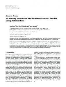
cluster is allocated a time slot. In the cluster steady phase, each member node sends data messages in its time slot at the idle state of a frame. In order to avoid collisions during communication, a kind of CSMA model is set up. In the steady phase, the final cluster-head collects the data acquired from the physical environment by all the members in its cluster and aggregates the data. Instead of transmitting the processed data to the base station directly, every cluster-head decides whether to choose another cluster-head as the next hop or not. Each cluster-head broadcasts its residual energy and position information to other cluster-heads. Then the clusterhead chooses the next hop using Dijkstra algorithm [14]. According to the result of computation, it decides whether to transmit the data to the base station directly or to send them to the next hop. The cluster-head allows the radio devices of each member to be turned off at all times, except during the transmission time. Data are sent from the cluster-head to the base station or next hop using a fixed spreading code and CSMA model. When a cluster-head has data to send to the base station (at the end of its frame), it must sense the channel to see if anyone else is transmitting data, using the base station spreading code. If so, the cluster-head waits to transmit the data. Otherwise, the cluster-head sends the data using the base station spreading code. The members communicate with their clusterhead using CSMA model to avoiding collisions. When one node drains its energy during its working time, it sends a death notification to the base station. Then the base station sends initialization notifications to all the nodes in the network. After receiving the initialization notifications, the network enters the cluster formation phase at the end of one round. If no node dies in the network, the network enters the cluster-head adjustment phase at the end of one round. In this phase, the cluster-head of last round will act as the auxiliary cluster-head, and every member node sends its position and residual energy information to it. After computation using BFOA by the auxiliary clusterhead, the new cluster-head in this round can be chosen out. As the working hours goes by, the sensor network enters one working phase after another. All the nodes are constructed into a cluster network. The base station collects the physical environment information from the nodes distributed in the specific area, after processing the data it transmits the compressed data to clients. Fig. 1 shows the time line of LEICP operation.

The second phase is very important among the three. The auxiliary cluster-head uses BFOA algorithm to compute the position of the final cluster-head in this phase. Then it sends notifications to all nodes in the cluster. Aiming at balancing the energy consumption among all the nodes and reducing energy dissipation of the cluster-head in the cluster a fitness function is proposed as follows: n λ 2 f (i ) = η ⋅ ei + ⋅ ∑ ⋅ ek ⋅ arctan d i k − d ave (7) n − 1 k =1, k ≠ i π n n 1 ⋅ ∑ ∑ dik , n(n − 1) i =1 k =1,k ≠i where η + λ = 1, η, λ ∈[0,1]. n is the number of nodes in the cluster. ei is the residual energy of the ith node. This function takes the residual energy and positions of nodes into consideration. It tries to balance the energy consumption in the cluster. According to this fitness function, the final clusterhead should be in such a position that the farther the member is from it, the more residual energy the member should own. The character of

d ave =

2

π

⋅ ek ⋅ arctan dik − dave

provides us this guarantee. Where ek is the residual energy of the kth node, dave is the average distance in a cluster and dik is the distance between the ith node and the kth node. When dik> dave, the larger dik is than dave, the larger the value of the function is. When dik< dave, the smaller dik is than dave, the larger the value of the function is. Let

u(dik ) =

2

π

⋅ ek ⋅ arctan dik − dave .

(8)

Supposing dave=29.2226, ek=0.25 and dik varies from 8.8299 to 45.2225, Fig. 2 shows the character of u(dik).

Fig. 2. u(dik)

In the cluster-head adjustment phase of every round, every node’s residual energy value can be regarded as a fixed value and dik is a variable. During the chemotactic steps, reproduction steps and elimination-dispersal events of bacteria (nodes), dik is changing. Let

u(ek ) = Fig. 1. Time line showing LEICP operation

1658

2

π

⋅ ek ⋅ arctan dik − dave

(9)

Supposing dave=29.2226, dik =45.2225 and ek varies from 0 to 0.25, u(ek) reflects a linearity character. Supposing dave=29.2226, dik=8.8299 and ek varies from 0 to 0.25, u(ek) reflects a similar characteristic to that when dik = 45.2225. According to the analysis we can know that if dik> dave or dik< dave, the larger the value of ek is, the larger the result of u(ek) is. If the distance value between the ith node and the kth node is a fixed value, the value of fitness function increases when the value of ek increases. In our research, we consider a sensor node a bacterium and a cluster a bacteria colony. Although all the nodes are immobile, in order to find the most suitable node to act as the final clusterhead we suppose that every bacterium could experience Run and Tumble, adjusting its position in the chemotactic processes. For every node, J (i) = f (i). (10) The second part of f (i),

λ

n −1

⋅

n

∑

k =1, k ≠ i

2

π

⋅ ek ⋅ arctan di k − d ave

Fig. 3. Paths for data transmission of cluster-heads

{vs,v1,v2…vp} is the set of cluster-heads of the sensor network. Node vt is the base station. Node vs is the source node. Node vs can choose another cluster-head as the next hop or send its data to Node vt directly. We present the data transmission network by a directed weighted graph D=(V, A), where V is a nonempty set of nodes (vertexes) and A is a set of arcs. vi and vj are two nodes in the graph. For the arc a=(vi, vj), w(a) = wij, which represents the weight of a. Here, wij represents the wasting energy of node vi. If node vi transfers data to node vj, wi j = l ⋅ Eelec + l ⋅ ε FS d ij 2 , if d ij < d 0 (12) = l ⋅ Eelec + l ⋅ ε TR d ij 4 , if d ij ≥ d 0

implies a cell-to-cell swarming process. The problem of finding the final cluster-head can be transformed into solving a maximum value problem. After a number of iteration loops the best bacterium with the most suitable position can be found. Then the most suitable where dij is the distance between vi and vj . If vj is the second position is mapped into one of the real positions of the nodes in hop node chosen by another cluster-head, vt is the base station, w jt = 2 ⋅ l ⋅ Eelec + l ⋅ ε FS d jt 2 , if d jt < d 0 the cluster. The node in this corresponding position will be (13) selected to be the final cluster-head. How is the most suitable = 2 ⋅ l ⋅ Eelec + l ⋅ ε TR d jt 4 , if d jt ≥ d 0 position mapped into one of the real position of the nodes in the because it includes a receiving consumption. cluster? An equation is given as follows: L is a path from node vs to node vt. The weight of L, w(L), is dmin = min{ Pb − P1 , Pb − P2 ⋅⋅⋅ Pb − Pi ⋅⋅⋅ Pb − Pn } (11) the sum of all the weights of arcs in L. The shortest path weight, 2 2 2 2 where P = { P1 , P2 ⋅⋅⋅ Pi ⋅⋅⋅ Pn } is the real position of n node in a also called distance, from node vs to node vt, denoted d(vs, vt) or dst, is the minimum weight of all possible directed paths with cluster, Pi = { X i , Yi } . P b = { X b , Y b } , which is the most suitable origin vs and destination vt. position after the adjustment using BFOA. The real position of In the specific steps of Dijkstra algorithm, we use Q and T to a certain node with dmin will be chosen to be the position of the represent the Q sign and T sign of some node. S represents the i final cluster-head, which means that the nearest node from the set of nodes with Q sign in the i step. In order to get the shortest Pb in the cluster will act as the final cluster-head. path and paths from node vs to other nodes we set the λ value After the cluster-heads aggregate the data they communicate for each node. When the algorithm comes to the end, λ(v)=m, it with each other in the steady phase of every round. Each one represents the front node of v is v in the shortest path from v m s broadcasts its position and compressed data information to to v. if λ(v)=M, it represents there is no path from v to v in D. if s other cluster-heads. After receiving the information, each λ(v)=0, which represents v= v . s cluster-head chooses the optimal route for transferring its data. For a directed weighted graph D=(V, A), the computation Dijkstra algorithm is a shortest path optimization algorithm, process is given in details. which is used by cluster-heads to choose the next hop. At the initial stage (i=0), S0={ vs }, Q(vs)=0, λ( vs)=0. To Fig. 3 shows the paths for data transmission of cluster-heads. every v, if v≠ vs, let T(v) = +∞, λ( v)=M, and k=s. Step 1: if Si=V, the algorithm ends and to every v∈ Si d(vs, v)= Q (v). Otherwise, go to Step 2. Step 2: Consider every vj , for which (vk, vj) ∈A and vj∉ Si. If T(vj)> Q (vk)+wkj, adjust T(vj) to be Q(vk)+wkj and λ( vj) to be k. Otherwise, go to Step 3.

1659

Step 3: Let T(vji) = min{T ( v j )} . v j ∉S i

If T(vji)