A Machine Learning Approach to Databases Indexes - ML Systems ...

A Machine Learning Approach to Databases Indexes

Alex Beutel, Tim Kraska∗, Ed H. Chi, Jeffrey Dean, Neoklis Polyzotis Google, Inc. Mountain View, CA {alexbeutel,kraska,edchi,jeff,npolyzotis}@google.com

Abstract Databases rely on indexing data structures to efficiently perform many of their core operations. In order to look up all records in a particular range of keys, databases use a BTree-Index. In order to look up the record for a single key, databases use a Hash-Index. In order to check if a key exists, databases use a BitMap-Index (a bloom filter). These data structures have been studied and improved for decades, carefully tuned to best utilize each CPU cycle and cache available. However, they do not focus on leveraging the distribution of data they are indexing. In this paper, we demonstrate that these critical data structures are merely models, and can be replaced with more flexible, faster, and smaller machine learned neural networks. Further, we demonstrate how machine learned indexes can be combined with classic data structures to provide the guarantees expected of database indexes. Our initial results show, that we are able to outperform B-Trees by up to 44% in speed while saving over 2/3 of the memory. More importantly though, we believe that the idea of replacing core components of a data management system through learned models has far reaching implications for future systems designs.2

1

Introduction

Whenever efficient data access is needed, index structures are the answer, and a wide variety of choices exist to address the different needs of various access pattern. For example, for range requests (e.g., retrieve all records in a certain timeframe) B-Trees are the best choice. If data is only looked up by a key, Hash-Maps are hard to beat in performance. In order to determine if a record exists, an existence index like a Bloom-filter is typically used. Because of the importance of indexes for database systems and many other applications, they have been extensively tuned over the last decades to be more memory, cache and/or CPU efficient [3, 5, 2, 1]. Yet, all of those indexes remain general purpose data structures, assuming the worst-case distribution of data and not taking advantage of more common patterns prevalent in real world data. For example, if the goal would be to build a highly tuned system to store and query fixed-length records with continuous integers keys (e.g., the keys 1 to 100M), one would not need to use a conventional B-Tree index over the keys since they key itself can be used as an offset, making it a constant O(1) rather than O(log n) operation to look-up any key or the beginning of a range of keys. Similarly, the index memory size would be reduced from O(n) to O(1). Of course, in most real-world use cases the data does not perfectly follow a known pattern, and it is usually not worthwhile to engineer a specialized index for every use case. However, if we could learn a model, which reflects the data patterns, correlations, etc. of the data, it might be possible to automatically synthesize an index structure, a.k.a. a learned index, that leverages these patterns for significant performance gains. In this paper, we explore to what extent learned models, including neural networks, can be used to replace traditional index structures from Bloom-Filters to B-Trees. This may seem counter∗ 2

Professor at Brown University, but work was done while at Google. A longer technical report, including more experiments, is available at alexbeutel.com/learned_indexes.

ML Systems Workshop at NIPS 2017, Long Beach, CA, USA.

intuitive because machine learning cannot provide the semantic guarantees we traditionally associate with these indexes, and because the most powerful machine learning models, neural networks, are traditionally thought of as being very expensive to evaluate. We argue that none of these obstacles are as problematic as they might seem with potential huge benefits, such as opening the door to leveraging hardware trends in GPUs and TPUs. We will spend the bulk of this paper explaining how B-Trees (§2), Hash maps (§3), and Bloom filters (§4) can be replaced with learned indexes. In Section 5, we will discuss how performance can be improved with recent hardware, learned indexes can be extended to support inserts, and other applications of this idea.

2

Range Index

Stage 3

Stage 2

Stage 1

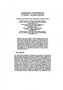
We begin with the case where we have an index that supports range queries. In this case, the data is stored in sorted order and an index is built to find the starting position of the range in the sorted array. Once the position at the start of the range is found, the database can merely walk through the ordered data until the end of the range is found. (We do not consider inserts or updates for now.) 2.1 Background The most common index structure for finding the position of a key in the sorted array is a B-Tree. B-Trees are balanced and cache-efficient trees. They differ from more common trees, like binary trees, in that at each node has a fairly large branching factor (e.g., 100) to match the page size for efficient memory hierarchy usage (i.e., the top-k nodes of the tree always remain in cache). As such, for each node that is processed, the model gets a precision gain of 100. Of course, processsing a node takes time. Typically, traversing a single node of size 100, assuming it is in cache, takes approximately 50 cycles to scan the page (we assume scanning, as it is usually faster than binary search at this size). 2.2 Learned Ranged Index At the core, B-Trees are models of the form f (key) → pos. We will use the more common machine learning notation where the key is represented by x and the position is y. Because we know all of the data in the database at training time (index construction time), our goal is to learn a model f (x) ≈ y. Interestingly, because the data x is sorted, f is modeling the cumulative distribution function (CDF) of data, a problem which has received some attention [4]3 . Key Model Architecture As a regression problem, we train our model f (x) with squared error to try to Model 1.1 predict position y. The question is what model architecture to use for f . As outline above, for the model … Model 2.1 Model 2.2 Model 2.3 to be successful, it needs to improve the precision of predicting y by a factor greater than 100 in a less … Model 3.1 Model 3.2 Model 3.3 Model 3.4 than 50 CPU cycles. With often many million of Position examples and needing high accuracy, building one large wide and deep neural network often gives not Figure 1: Staged models very strong accuracy while being expensive to execute. Rather, inspired by the mixture of experts work [6], we build a hierarchy of models (see Figure 1). We consider that we have y ∈ [0, N ) and at stage ` there are M` models. We train the model at (k) stage 0, f0 (x) = y. As such, model k in stage `, denoted by f` , is trained with loss: L` =

X

(f`−1 (x))

(f`

(x) − y)2

L0 =

(x,y)

X

(f0 (x) − y)2

(x,y)

(f

(x))

`−2 Note, we use here the notation here of f`−1 (x) recursively executing f`−1 (x) = f`−1 (x). Therefore, in total, we iteratively train each stage with loss L` to build the complete model. Interestingly, we find that it is necessary to train iteratively as Tensorflow has difficulty scaling to computation graphs with tens of thousands of nodes. Constraints Unlike typical ML models, it is not good enough to return the approximate solution. Rather, at inference time, when the model produces an estimate of the position, we must find the actual record that corresponds to the query key. Traditionally, B-Trees provide the location of the beginning of the page where the key lies. For learned indexes, we need to search around the prediction, to actually find the beginning of the range.

Interestingly, we can easily bound the error of our model such that we can use classic search algorithms like binary search. This is possible because we know at training time all keys the model is 3

This assumes records are fixed-length. If not, the function is not the CDF, but another monotonic function.

2

indexing. As such, we can compute the maximum error ∆ the model produces over all keys, and at inference time perform a search in the range [ˆ y − ∆, yˆ + ∆]. Further, we can consider the model’s error over subsets of the data. For each model k in the last stage of our overall model, we compute its error ∆k . This turns out to be quite helpful as some parts of the model are more accurate than others, and as the ∆ decreases, the lookup time decreases. An interesting future direction is to minimize worst-case error ∆ rather than average error. In some cases, we have also built smaller B-Trees to go from the end of the model predictions to the final position. These hybrid models are often less memory efficient but can improve speed due to cache-efficiency. Total Model Search Size Size Type Config Speedup 2.3 Experiments (ns) (ns) (ns) (MB) Savings We have run experiments on 200M web-log B-Tree page size: 64 274 169 105 4% 24.92 100% page size: 128 263 131 131 0% 12.46 0% records with complex patterns created by page size: 256 271 117 154 3% 6.23 -50% school holidays, hourly-variations, special Learned 2nd stage size: 10,000 178 26 152 -32% 0.15 -99% Index 2nd stage size: 50,000 162 35 127 -38% 0.76 -94% events etc. We assume an index over the 2nd stage size: 100,000 152 36 116 -42% 1.53 -88% timestamps of the log records (i.e., an index 2nd stage size: 200,000 146 40 106 -44% 3.05 -76% over sorted, unique 32bit timestamps). We Figure 2: Performance learned index vs B-tree. used a cache-optimized B-Tree with a pagesize of 128 as the baseline, but also evaluated other page sizes. As the learned range index we used a 2-stage model (1st stage consist of 1 linear model, 2nd stage consist of varying number of linear models). We evaluated the indexes on an Intel-E5 CPU with 32GB RAM without a GPU/TPU. Results of our experiments can be seen in Figure 2. We find that learned indexes are significant faster than B-Tree models while using much less memory. This results is particular encouraging as the next generation of TPUs/GPUs will allow to run much larger models in less time.

3

Point Index

If access to the sorted items is not required, point indexes, such as hash-maps, are commonly used. The hash map works by taking a function h that maps h(x) → pos. Traditionally, a good hash function is one for which there is no correlation between the distribution of x and positions. We consider placing our N keys in an array with m positions. Two keys can be mapped to the same position, with probability defined by the birthday paradox, and in this case a linked list of keys is formed at this location. Collisions are costly because (1) latency is increased walking through the linked list of collided items, and (2) many of the m slots in the array will be unused. Generally the latency and memory are traded-off through setting m. 3.1 Learned Point Index Again, we find that using the distribution of keys to be useful in improving hash map efficiency. If we knew the CDF of our data, then an optimal hash would be h(x) = mCDF(x), resulting in no collisions and no empty slots when m = N . Therefore, as before, we can train a model f (x) to approximate the CDF and use this model as our hash function. 3.2 Experiments We tested this technique on the 200M web-log dataset by using the 2-stage model with 100,000 models in the second stage as in Sec. 2.3. For a baseline we use a random hash function. Setting m = 200M, we find that the learned index results in a 78% space improvement as it causes less collisions and thus, linked-list overflows, while only being slightly slower in search time (63ns as compared to 50ns). Across other datasets and settings of m we generally find an improvement in memory usage with a slight increase in latency.

4

Existence Index

Existence indexes are important to determine if a particular key is in our dataset, such as to confirm its in our dataset before retrieving data from cold storage. Therefore, we can think of an existence index as a binary classification task where one class is that the key is in our dataset and the other class is everything not in the dataset.

Key

Model Yes

No

Bloom filter Yes

Bloom filters have long been used as an efficient way to check if a particular item exists in a dataset. They provide the guarantee there will be no false negatives (any item in the dataset will return True from the Figure 3: BF as a classifier model), but there can be some false positives. This is done by taking a bit array M of length m and taking k different hashes of the key. We set M [fk (x) mod m] = 1 for all keys x and for all hash functions k. Then, at inference time, if any of the bits M [fk (x) mod m] are set to 1, then we return that the key is in the dataset. 3

We can determine m and k based on a desired false positive rate p: m = (n ln p)/(ln 2)2 and k = − log2 p. Importantly, the size of the bitmap grows linearly with the number of items in the dataset, independent of their data distribution. 4.1 Learned Existence Index While bloom filters make no assumption about the distribution of keys, nor the distribution of false queries against the bloom filter, we find we can get much better results by learning models that do make use of those far from random distributions. Modeling The job of an existence index can be framed as a binary classification task, where all items in the dataset have a label of 1 and all other possible inputs have a label of 0. We consider x to be strings, and train simple RNNs and CNNs with a sigmoid prediction, denoted by f (x), with logistic loss. While we have focused on using well-defined query sets (e.g., previous queries against a bloom filter) as our negative class, recent work on GAN-based text generation could provide a more robust way of training learned bloom filters. No False Negatives One of the key challenges in learned existence indexes is that at inference time we cannot have false negatives. We address this by building an “overflow” bloom filter. That is, for all keys x in our dataset for which f (x) < τ , we insert x into a bloom filter. We set our threshold τ so that the false positive rate over our query set matches p. One advantage of this approach is that our overflow bloom filter scales with the false negative rate (FNR) of our model. That is, even if our model has a FNR of 70%, it will reduce the size of the bloom filter by 30% because bloom filters scale with the number of items in the filter. 4.2 Experiments We explore the application of an existence index for blacklisted phishing URLs. We use data from Google’s transparency report with 1.7M unique phishing URLs. We use a negative set that is a mixture of random (valid) URLs and whitelisted URLs that could be mistaken for phishing pages. A normal bloom filter with a desired 1% false positive rate requires 2.04MB. Using an RNN model of the URLs, a false positive rate of 1% has a true negative rate of 49%. With the RNN only using 0.0259MB, the total existence index (RNN model + spillover bloom filter) uses 1.07MB, a 47% reduction in memory.

5

Future Directions and Conclusion

In this paper, we have laid out the potential for using machine learned models as indexes in databases. We believe this perspective opens the door for numerous new research directions: • Low-Latency Modeling: The latency needed for indexes is in the nanoseconds not milliseconds as for other models. There are unique opportunities to develop new types of low-latency models that take better advantage of GPUs and TPUs and the CPU cache. • Multidimensional data: ML often excels at modeling multidimensional data, while database indexes have difficulty scaling in the number of dimensions. Learning models for multidimensional indexes or efficient joins would provide additional benefit to databases. • Inserts: We have focused on read-only databases. In the case of inserts, databases often use spillover data structures and then “rebuild” (train) their indexes intermittently. Using online learning or building models which generalize, not just overfit, should make it possible for learned indexes to handle inserts, and deserves further study. • More algorithms: We believe this perspective can provide benefits to other classical algorithms. For example, a CDF model could improve the speed of sorting. As we have demonstrated, ML models have the potential to provide significant benefits over state-ofthe-art database indexes, and we believe this is a fruitful direction for future research. Acknowledgements We would like to thank Chris Olston for his feedback during the development of this work.

References [1] K. Alexiou, D. Kossmann, and P.-A. Larson. Adaptive range filters for cold data: Avoiding trips to siberia. Proc. VLDB Endow., 6(14):1714–1725, Sept. 2013. [2] B. Fan, D. G. Andersen, M. Kaminsky, and M. D. Mitzenmacher. Cuckoo filter: Practically better than bloom. In Proceedings of the 10th ACM International on Conference on Emerging 4

Networking Experiments and Technologies, CoNEXT ’14, pages 75–88, New York, NY, USA, 2014. ACM. [3] G. Graefe and P. A. Larson. B-tree indexes and cpu caches. In Proceedings 17th International Conference on Data Engineering, pages 349–358, 2001. [4] M. Magdon-Ismail and A. F. Atiya. Neural networks for density estimation. In M. J. Kearns, S. A. Solla, and D. A. Cohn, editors, Advances in Neural Information Processing Systems 11, pages 522–528. MIT Press, 1999. [5] S. Richter, V. Alvarez, and J. Dittrich. A seven-dimensional analysis of hashing methods and its implications on query processing. Proc. VLDB Endow., 9(3):96–107, Nov. 2015. [6] N. Shazeer, A. Mirhoseini, K. Maziarz, A. Davis, Q. Le, G. Hinton, and J. Dean. Outrageously large neural networks: The sparsely-gated mixture-of-experts layer. arXiv preprint arXiv:1701.06538, 2017.

5