Feb 9, 2008 - arXiv:nucl-th/9505022v1 17 May 1995. A method of calculating the Jost function for analytic potentials. S. A. Rakityanskyâ, S. A. Sofianos, and ...
A method of calculating the Jost function for analytic potentials S. A. Rakityansky∗ , S. A. Sofianos, and K. Amos∗∗
arXiv:nucl-th/9505022v1 17 May 1995
Physics Department, University of South Africa, P.O.Box 392, Pretoria 0001, South Africa (February 9, 2008)
Abstract A combination of the variable-constant and complex coordinate rotation methods is used to solve the two-body Schr¨ odinger equation. The latter is replaced by a system of linear first-order differential equations, which enables one to perform direct calculation of the Jost function for all complex momenta of physical interest, including the spectral points corresponding to bound and resonance states. Explicit forms of the equations, appropriate for central, noncentral, and Coulomb-tailed potentials are given. Within the proposed method, the scattering, bound, virtual, and resonance state problems can be treated in a unified way. The effectiveness of the method is demonstrated by a numerical example. PACS numbers: 03.65.Nk, 21.45.+v, 02.70.+d I. INTRODUCTION
The nonrelativistic quantum mechanical two-body problem can be described conveniently and nicely in terms of the Jost functions and Jost solutions of the Schr¨odinger equation. When defined for all complex values of the momentum, these functions contain complete information about the underlying physical system. In contrast to the conventional treatment of the two-body problem, based on the scattering amplitude and physical wave-function, in the Jost function approach the bound, virtual, scattering, and resonance states are treated on an equal footing and simultaneously. Also the Jost function is a more fundamental quantity than the S function since it is free of ambiguities caused by redundant zeros, while the S function may have redundant poles [1]. Despite the fact that the Jost functions are more appropriate, in principle, for studies of spectral properties of two-body Hamiltonians, they have not been used in the past in practical calculations. Instead they were considered as purely mathematical entities of formal scattering theory, which can be expressed either via an integral containing the regular solution or via a Wronskian of the regular and Jost solutions [2]. Thus, to find the Jost function based upon such information, the full solution of the problem itself is required. In Ref. [3], linear first-order differential equations for functions closely related to the Jost solutions were proposed. These equations are based on the variable-phase approach [4] and their solution at any fixed value of the radial variable r, provides the Jost function and its complex conjugate counterpart, which correspond to the potential truncated at the point r.
1
The proposed method, however, is suitable only for bound and scattering states calculations, that is for calculations in the upper half of the complex momentum plane. Herein we extend the method of Ref. [3] onto the unphysical sheet so that the resonance state region is included. We do so by a combination of the variable-constant method [5] and the ‘complex coordinate rotation’ method [6]. The latter method, often used in studies of atomic and molecular physics, is also known as the ’complex-scaling’ or the ‘complexdilation’ method. It is based on the fact that the complex coordinate transformation, ~r → ~r exp(iθ) with a sufficiently large θ > 0, makes the resonance state wave function quadratically integrable leaving the energies and widths of the bound and resonance states unaffected since the Jost function, and the positions of its zeros in particular, do not depend on that vector ~r. This is true if the potential is an analytic function of the coordinate r and vanishes rapidly enough when that coordinate goes to infinity along the turned ray [2]. In atomic and molecular physics, this property has been used to locate resonances by the same variational methods employed for the bound states [7]. In this paper we make a complex rotation of the radial variable in the differential equations proposed in Ref. [3]. The new equations that result, facilitate evaluation of the Jost function in the entire complex momentum plane and therefore one can locate the resonances as the zeros of the Jost function. The paper is organized as follows. In Sec. II we derive the rotated equations in the simplest case of a central short–range potential. In Sec. III the equations are generalised for the case of a noncentral potential, while Sec. IV is devoted to consideration of potentials having a Coulomb tail. In Sec. V the method is tested by comparing results with the properties of an exactly solvable model. Finally, possible further extensions of the method, its advantages and drawbacks are discussed in Sec. VI. II. CENTRAL SHORT–RANGE POTENTIAL
Consider the problem of two quantal particles interacting via a central potential V (r) with the asymptotic properties lim r 2 V (r) = 0 ,
(1)
r→0
and lim r 1+ε V (r) = 0 ,
r→∞
ε>0.
(2)
Any physical solution of the radial Schr¨odinger equation (¯ h = 2m = 1) Dℓ (k, r) Φℓ (k, r) = V (r) Φℓ (k, r) ,
(3)
Dℓ (k, r) ≡ ∂r2 + k 2 − ℓ(ℓ + 1)/r 2 ,
(4)
where
is proportional to the so-called regular solution which is defined by the boundary condition at the origin, 2
lim [Φℓ (k, r)/ℓ(kr)] = 1 .
(5)
r→0
Here ℓ (z) is the Riccati-Bessel function [8]. At large distances the regular solution is a (±) linear combination [9] of Riccati-Hankel functions hℓ (kr) [8], i.e. i 1 h (+) (−) hℓ (kr) fℓ∗ (k ∗ ) + hℓ (kr) fℓ (k) , 2
Φℓ (k, r) −→
r→∞
(6)
wherein the r−independent quantity fℓ (k) is the Jost function whose zeros in the complex k–plane correspond to the bound, (Re k = 0, Im k > 0 ), virtual, (Re k = 0, Im k < 0 ), and resonance, (Re k > 0, Im k < 0 ), states of the system. Suppose V (r) is an analytic potential [2], i.e. it can be defined as an analytic function of the complex variable r = x exp(iθ),
x ≥ 0,
θ ∈ [0, θmax ],
θmax < π/2 ,
(7)
and fulfills the conditions of Eqs. (1) and (2). We consider the complex dilation of the regular solution using this rotated coordinate. The corresponding function Φℓ (k, xeiθ ) is square integrable over the variable x, even for a resonance state, provided the angle θ is greater than ϕ which defines the position of the resonance on the lower half of the complex k-plane by k0 = |k0 | exp(−iϕ).
(8)
This is obvious because the product ‘k0 r’ in the asymptotic behaviour ∼ exp(ik0 r) of the solution has a positive imaginary part. To obtain the equation for the dilated regular solution, we substitute Eq. (7) into Eqs. (3) and (5) giving Dℓ (keiθ , x) Φℓ (k, xeiθ ) = e2iθ V (xeiθ ) Φℓ (k, xeiθ ) ,
(9)
and h
.
i
lim Φℓ (k, xeiθ ) jℓ (kxeiθ ) = 1 .
x→0
(10)
Furthermore, and since the potential is assumed to be analytic, substitution of Eq. (7) into Eq. (6) gives the asymptotic form Φℓ (k, xeiθ ) −→
x→∞
i 1 h (+) (−) hℓ (kxeiθ ) fℓ∗ (k ∗ ) + hℓ (kxeiθ ) fℓ (k) . 2
(11)
Note that the Jost functions in Eqs. (6) and (11) are the same because the Jost function does not depend on the rotation angle θ. Hence, the positions of its zeros are θ-independent as well. To solve the differential equation, Eq. (9), we apply the variable constant method [5], i.e. we look for a solution in the form Φℓ (k, xeiθ ) =
i 1 h (+) (+) (−) (−) hℓ (kxeiθ ) Fℓ (k, x, θ) + hℓ (kxeiθ ) Fℓ (k, x, θ) , 2
3
(12)
which is an r–dependent combination of two linearly independent solutions of the free equation (±)
Dℓ (keiθ , x) hℓ (kxeiθ ) = 0.
(13) (±)
Instead of one unknown function Φℓ , we have introduced two unknown functions Fℓ which necessitates an additional constraint condition. The most convenient is the standard Lagrange condition [5] (+)
(+)
(−)
(−)
hℓ (kxeiθ ) ∂x Fℓ (k, x, θ) + hℓ (kxeiθ ) ∂x Fℓ (k, x, θ) = 0 ,
(14)
which makes ∂x Φℓ continuous even if the potential has a sharp cut-off at a point x = x0 . Substituting this ansatz, Eq. (12), into Eq. (9) and using Eqs. (13) and (14), lead to coupled differential equations (+) ∂x Fℓ (k, x, θ)
and (−) ∂x Fℓ (k, x, θ)
eiθ (−) = hℓ (kxeiθ ) V (xeiθ ) 2ik h i (+) (+) (−) (−) × hℓ (kxeiθ ) Fℓ (k, x, θ) + hℓ (kxeiθ ) Fℓ (k, x, θ) , eiθ (+) =− hℓ (kxeiθ ) V (xeiθ ) 2ik h i (+) (+) (−) (−) × hℓ (kxeiθ ) Fℓ (k, x, θ) + hℓ (kxeiθ ) Fℓ (k, x, θ) ,
(15)
(16)
with boundary conditions
(+)
(−)
Fℓ (k, 0, θ) = Fℓ (k, 0, θ) = 1 ,
(17)
that follow immediately from Eqs. (10) and (12). With these boundary conditions, this system of coupled differential equations are equivalent to the pair of integral Volterra-type equations, (+)
Fℓ (k, x, θ) = 1 +
eiθ ik
Z
x
(−)
hℓ (kx′ eiθ )V (x′ eiθ )Φℓ (k, x′ eiθ ) dx′ ,
(18)
eiθ Z x (+) h (kx′ eiθ )V (x′ eiθ )Φℓ (k, x′ eiθ ) dx′ . ik 0 ℓ
(19)
0
and (−)
Fℓ (k, x, θ) = 1 −
Iterated solution of these equations, on a small interval [0, xmin ] and with ℓ (kxeiθ ) as the zero-order approximation to Φℓ (k, xeiθ ), can be used to obtain the boundary values (±) Fℓ (k, xmin , θ), which in turn are needed to solve the differential equations, Eqs. (15) and (16), numerically. Thus, we can find the complex dilation Φℓ (k, xeiθ ) of the regular solution in the form Eq. (12), using either differential (Eqs. (15) and (16)) or integral (Eqs. (18) and (19)) equations. The question then arises as to the physical meaning of this solution and that of the (±) functions Fℓ (k, x, θ). To answer, we note that the complex rotation, Eq. (7), makes the 4
Hamiltonian nonhermitian, so it can have complex eigenvalues [10]. Indeed, the Jost function can have zeros, not only on the imaginary axis of the (complex) k-plane but also in the entire lower half of that plane. Schematically this is depicted in Fig. 1. Therein, the points on the positive imaginary axis (k01 , k02 , k03 ) represent Jost function zeros corresponding to physical bound states of the system. The points shown in the fourth quadrant (k04 , k05 ), are the resonance state zeros. The dividing line defined by the rotating angle θ is also displayed. This line is the limit for the resonance position angle ϕ for which the condition Im kr > 0 is fulfilled. The asymptotic form of the function Φℓ (k0 , xeiθ ), corresponding to these zeros, decreases exponentially if the angle θ is chosen large enough, i.e. greater than the angle ϕ of Eq. (8), since [8] (±)
hℓ (kxeiθ ) −→ ∓i exp[±i(kxeiθ − x→∞
ℓπ )]. 2
(20)
Hence Φℓ (k0 , xeiθ ) are square-integrable eigenfunctions of the rotated Hamiltonian corresponding to either real (bound) (Re k0 = 0, Im k0 > 0) or complex (Re k0 > 0, Im k0 < 0) eigenvalues. Although these eigenvalues, being independent of θ, always correspond to the energies of the physical bound and resonance states, the corresponding solutions Φℓ (k0 , xeiθ ) acquire physical meaning only when θ = 0. However, if one is interested only in eigenenergies, it is convenient to use θ > 0 thereby dealing with square-integrable wave functions. This idea was successfully used for the location of resonances with variational methods [6]. In the present approach, the square-integrable nature of the dilated regular solution at resonance energies is not used directly. Instead, the crucial feature for our approach is that (+) the function hℓ (kxeiθ ) decreases exponentially at large x if Im (kxeiθ ) > 0. This is true for the whole region of the complex k-plane in which the bound and resonance state zeros lie (see Fig. 1). In contrast, the regular solution is square integrable only at the discrete points k0i of this region. According to Eq. (11), at all other points k not coinciding with the spectrum k0i of the rotated Hamiltonian, the regular solutions diverge as iθ Φℓ (k, xeiθ ) ∼ e|Im (kxe )| .
(21) (±)
As can be seen from Eqs. (18) and (19), both functions Fℓ finite limits when x → ∞ (+)
∗ lim Fℓ (k0i , x, θ) = fℓ∗ (k0i ),
x→∞
at the spectral points k0i , have (22)
and (−)
lim Fℓ (k0i , x, θ) = fℓ (k0i ) = 0 ,
x→∞
(23)
which must coincide with the asymptotic coefficients defined in Eq. (11). At any other point k 6= k0i within the zone Im (kxeiθ ) > 0, the integral of Eq. (19) still has a finite limit, (−)
lim Fℓ (k, x, θ) = fℓ (k) ,
x→∞ (+)
(24)
because hℓ (kxeiθ ) is a decreasing function. However, the integral in Eq. (18) diverges. This is not surprising and by no means a defect to our approach. Simply, it reflects the 5
(±)
well-known fact (see, for example, Refs. [2] and [11]) that the Jost solutions, Fℓ (k, r), of the Schr¨odinger equation with boundary conditions, (±)
lim e∓ikr Fℓ (k, r) = 1 ,
(25)
r→∞
(+)
are defined within different regions of the complex k-plane : Im k ≤ 0 for Fℓ and Im k ≥ 0 (−) for Fℓ . The only common region of their definition is the real axis Im k = 0 i.e. the physical region. Only for a special class of rapidly decreasing potentials it would be a band along this axis [2,9,11]. However here we consider the most general case defined by the condition Eq. (2). (±) The same is true for the limit (x → ∞) of our functions Fℓ (k, x, θ) with θ = 0, which are closely related to the Jost solutions, as one can see from Eq. (12). However, in contrast (±) to the Jost solutions, the functions Fℓ (k, x, 0) are well defined for any finite x, because the boundary conditions, Eq. (17), are imposed on them at the point x = 0. When θ > 0, the border dividing the two regions of complex k where the limits of (±) Fℓ (k, x, θ) exist, is rotated downwards to the line |k|e−iθ . The fact that above this line the (+) function Fℓ (k, x, θ) has no limit for x → ∞ does not contradict the asymptotic requirement of Eq. (11). Written in general form, these asymptotics must include both terms, (+)
hℓ (kxeiθ )fℓ∗ (k ∗ )
and
(−)
hℓ (kxeiθ )fℓ (k),
only on the dividing line, Im (kxeiθ ) = 0, where they are of the same order of magnitude. Above this line, Eq. (11) is a sum of ‘small’ and ‘large’ terms; the first of which can be (+) omitted. The ‘small’ term, hℓ (kxeiθ )fℓ∗ (k ∗ ), becomes significant above the dividing line (−) only at the discrete points k = k0i , i = 1, 2, . . . , N where the ‘large’ term, hℓ (kxeiθ )fℓ (k), disappears because fℓ (k0i ) = 0. And, as we have already seen, at these points the limit Eq. (22) exists and the ‘small’ term is well defined. At all other points the growth of (+) (+) Fℓ (k, x, θ) is suppressed by the exponentially decreasing factor hℓ (kxeiθ ) and the ‘small’ term becomes negligible as compared to the ‘large’ term. Indeed, at a sufficiently large x the integrand of Eq. (18) behaves like ∼ exp(−2ikxeiθ )V (xeiθ ). (+)
If the potential at infinity is a nonzero constant, then the integration would produce Fℓ ∼ (+) exp(−2ikxeiθ ). However, the potential obeys the condition Eq. (2) so that Fℓ diverges (+) (+) less rapidly than exp(−2ipxeiθ ). Therefore the product hℓ Fℓ grows less rapidly than (−) hℓ (kxeiθ ) and does not affect the asymptotic properties specified by Eq. (11). The twoterm decomposition, Eq. (12), guarantees term by term correspondence with the asymptotic form Eq. (11) at the discrete points k0i and also on the dividing line Im (kxeiθ ) = 0. For the other points (k 6= k0i , Im (kxeiθ ) > 0), the first term of Eq. (12) contains some admixture dℓ (k, x, θ) of the diverging term. However, this admixture is infinitesimal as compared to (−) the leading term, hℓ (kxeiθ )fℓ (k) of the long range asymptotic behaviour, Φℓ (k, x, θ) x→∞ −→
o 1 n (+) (−) [hℓ (kxeiθ )fℓ∗ (k ∗ ) + dℓ (k, x, θ)] + hℓ (kxeiθ )fℓ (k) , 2
6
(26)
i.e. n
(+)
.
(−)
o
lim [hℓ (kxeiθ )fℓ∗ (k ∗ ) + dℓ (k, x, θ)] hℓ (kxeiθ )fℓ (k) = 0 .
x→∞
(+)
(27)
(−)
The asymptotic behaviour of the functions Fℓ (k, x, θ) and Fℓ (k, x, θ) below the dividng (+) (−) line |k|e−iθ is just the opposite, i.e. Fℓ is finite and Fℓ diverges. However, the function (−) (+) Fℓ (k, x, θ) has a physical content only when Im (kxeiθ ) ≥ 0, while Fℓ (k0i , x, θ) at the (−) discrete points k0i , i = 1, 2, . . . , N, where Fℓ (k0i , ∞, θ) = 0. Thus, if the potential permits a large enough choice for θ, we can calculate the Jost function for all complex values of k 6= 0 of interest, including the momenta on the positive imaginary axis and in the resonance region under the positive real axis as well. As a consequence of Eq. (24), the Jost function can be found by solving the coupled one–dimensional equations, Eqs. (15) and (16), from x = 0 to x = xmax , where xmax is determined by the required accuracy and on how fast the potential decreases. The faster it decreases the sooner (−) (−) ∂x Fℓ (k, x, θ) vanishes and Fℓ (k, x, θ) tends smoothly to the constant fℓ (k). It is interesting to note that at sufficiently large x the system of equations, Eqs. (15) (+) (+) and (16), decouple as the ‘small’ term hℓ Fℓ becomes insignificant as compared to the (−) (−) ‘large’ term hℓ Fℓ . III. NONCENTRAL SHORT–RANGE POTENTIAL
In this section we consider a two-body problem with spin-dependent interaction which does not conserve the orbital angular momentum ℓ. As in the previous section, we assume that the matrix elements JM JM JM r )|Yℓs > V(JM ℓ′ s′ ),(JM ℓs) (r) ≡< Yℓ′ s′ |V (~
of the potential operator, sandwitched between the spin-angular momentum eigenfunctions JM Yℓs (ˆ r) ≡
X
JM Cℓmsµ Yℓm (ˆ r)χsµ
mµ
of the total angular momentum operator, J~ = ~ℓ + ~s, obey the same constraints (1) and (2) at the origin and infinity. To simplify the notation, the superscripts JM will be omitted and instead of the pair of subscripts ℓs, satisfying the triangle condition |J − s| ≤ ℓ ≤ |J + s|, we will use the symbol [ℓ].
7
A. Boundary conditions
The physical wave-function, describing the state with a given momentum ~k, is the product 1 1 X JM Ψ(~k, ~r) = (Y · u) ≡ Y (ˆr)u[ℓ](~k, r) r r [ℓ] ℓs of the [ℓ]–row of Y and the [ℓ]–column u of the radial components satisfying the coupled differential equations Dℓ (k, r)u[ℓ](~k, r) =
X
V[ℓ][ℓ′] (r)u[ℓ′] (~k, r)
(28)
[ℓ′ ]
with (physical) boundary conditions u[ℓ] (~k, 0) = 0, (29) u[ℓ] (~k, r) −→ U[ℓ] (~k, r), r→∞
where the asymptotic function U[ℓ] (~k, r) has a different form for the bound, scattering, and resonance states. As it is more convenient to deal with universal boundary conditions imposed at a single point, we consider the so-called fundamental matrix, Φ[ℓ′ ][ℓ] (k, r), of the regular solutions instead of the physical column solution, u[ℓ](~k, r). The physical solution then can be constructed as a linear combination of columns of Φ[ℓ′ ][ℓ] (k, r). By definition, Φ is a fundamental matrix if it has the following three properties [2]: i) Each column of Φ[ℓ′ ][ℓ] is a solution of Eq. (28), i.e Dℓ (k, r) Φ[ℓ][ℓ′] (k, r) =
X
V[ℓ][ℓ′′] (r) Φ[ℓ′′ ][ℓ′] (k, r) ,
(30)
[ℓ′′ ]
ii) Φ[ℓ′ ][ℓ] (k, 0) = 0, and iii) all columns of Φ[ℓ′ ][ℓ] are linearly independent. Moreover, Φ[ℓ′ ][ℓ] must be a square matrix since Eq. (28) has as many independent regular solutions as the column dimension [12]. The property ii) implies that the desired universal boundary condition should be imposed at the point r = 0. We emphasize here that the boundary condition Φ[ℓ′ ][ℓ](k, 0) = 0, is not sufficient to define this matrix since Eq. (30) is of second order. Furthermore, Eq. (18) is singular at the origin, and consequently the existence and uniqueness theorem [12] is not valid at this point. However, this theorem is valid for any small r ≥ δ > 0. Hence, the matrix Φ can be uniquely defined by Φ(k, δ) and ∂r Φ(k, δ), while within the interval [0, δ], Φ(k, r) can be evaluated explicitly as follows. After multiplying by r 2 and using Eq. (1), Eqs. (30) decouple giving h
i
r 2 ∂r2 − ℓ(ℓ + 1) Φ[ℓ][ℓ′] (k, r) = 0, 8
r ∈ [0, δ] .
(31)
Each of these equations has two independent solutions, namely the functions ∼ r ℓ+1 and ∼ r −ℓ . Therefore, near the origin, we can use the Riccati-Bessel function, √ ℓ+1 πk ℓ (kr) −→ ℓ+1 r ℓ+1 , (32) r→0 2 Γ(ℓ + 32 ) as the regular solution. Hence, as a first order approximation to Φ[ℓ][ℓ′ ] (k, r) for r ∈ [0, δ] we can take the diagonal matrix Φ[ℓ][ℓ′] (k, r) ∼ δ[ℓ][ℓ′] ℓ′ (kr) , r→0
(33)
satisfying the above-mentioned three properties. Higher order corrections give non–zero off-diagonal elements, so to guarantee linear independence of the columns, the off-diagonal elements of a row must be infinitesimal in comparison to the diagonal element of that row. The boundary condition thus reads Φ[ℓ][ℓ′ ] (k, r) = δ[ℓ][ℓ′] , r→0 ℓ′ (kr) lim
(34)
which is a generalization of Eq. (5). Since Φ is the fundamental matrix, any physical solution is a linear combination of its columns with r-independent coefficients, i.e. u[ℓ] (~k, r) =
X
Φ[ℓ][ℓ′] (k, r)A[ℓ′] (~k) .
(35)
[ℓ′ ]
The coefficients A[ℓ] must be chosen to satisfy the appropriate boundary condition (29) at infinity. B. Complex rotation
To generalize the approach described in the previous section, we perform the complex rotation, Eq. (7), of the coordinate. The corresponding complex dilation of the fundamental matrix, Φ[ℓ][ℓ′] (k, xeiθ ), is the solution of Dℓ (keiθ , x) Φ[ℓ][ℓ′] (k, xeiθ ) = e2iθ
X
V[ℓ][ℓ′′] (xeiθ ) Φ[ℓ′′ ][ℓ′ ] (k, xeiθ ) ,
(36)
[ℓ′′ ]
where h
i
.
lim Φ[ℓ][ℓ′] (kxeiθ ) jℓ′ (kxeiθ ) = δ[ℓ][ℓ′ ] .
x→0
(37)
We then apply the variable-constant method i.e. look for a solution of the form Φ[ℓ][ℓ′] (k, xeiθ ) =
i 1 h (+) (+) (−) (−) hℓ (kxeiθ ) F[ℓ][ℓ′] (k, x, θ) + hℓ (kxeiθ ) F[ℓ][ℓ′] (k, x, θ) , 2
with 9
(38)
(+)
(+)
(−)
(−)
hℓ (kxeiθ ) ∂x F[ℓ][ℓ′] (k, x, θ) + hℓ (kxeiθ ) ∂x F[ℓ][ℓ′] (k, x, θ) = 0 .
(39)
(±)
The resulting coupled equations for the new unknown functions, F[ℓ][ℓ′] (k, x, θ), have the form X eiθ (−) hℓ (kxeiθ ) V[ℓ][ℓ′′] (xeiθ ) 2ik [ℓ′′ ]
(+)
∂x F[ℓ][ℓ′] (k, x, θ) =
h
(+)
(+)
(−)
(−)
i
(40)
(−)
(−)
i
(41)
× hℓ′′ (kxeiθ )F[ℓ′′ ][ℓ′ ] (k, x, θ) + hℓ′′ (kxeiθ )F[ℓ′′ ][ℓ′] (k, x, θ) , and (−)
∂x F[ℓ][ℓ′] (k, x, θ) = −
X eiθ (+) hℓ (kxeiθ ) V[ℓ][ℓ′′] (xeiθ ) 2ik [ℓ′′ ] h
(+)
(+)
× hℓ′′ (kxeiθ )F[ℓ′′ ][ℓ′] (k, x, θ) + hℓ′′ (kxeiθ )F[ℓ′′ ][ℓ′] (k, x, θ) .
The appropriate boundary conditions for them can be derived from Eqs. (37) and (38). First (+) (−) though, one must compensate the singularities of hℓ (kxeiθ ) and hℓ (kxeiθ ) at x = 0. For this we can demand F (+) and F (−) to be identical as x → 0, viz. (+)
F[ℓ][ℓ′] (k, x, θ) ∼ F[ℓ][ℓ′] (k, x, θ) , x→0
(42)
and (−)
F[ℓ][ℓ′] (k, x, θ) ∼ F[ℓ][ℓ′] (k, x, θ) ,
(43)
Φ[ℓ][ℓ′] (k, xeiθ ) ∼ ℓ (kxeiθ ) F[ℓ][ℓ′] (k, x, θ) ,
(44)
x→0
as then x→0
so that, from Eq. (37), the boundary conditions become h
(±)
.
i
lim ℓ (kxeiθ )F[ℓ][ℓ′] (k, x, θ) ℓ′ (kxeiθ ) = δ[ℓ][ℓ′] .
x→0
(45)
However, as x = 0 is a singular point, for practical calculations one needs to solve Eqs. (40) and (41) analytically on a small interval (0, δ] and then impose the boundary conditions at x = δ. Such an analytical solution can be found easily by choosing δ to be small enough so that for x ∈ (0, δ] we can write (±)
∂x F[ℓ][ℓ′] (k, x, θ) = ± (±)
For small x, in hℓ
eiθ (∓) h (kxeiθ ) V[ℓ][ℓ′] (xeiθ ) ℓ′ (kxeiθ ) . ik ℓ
(46)
≡ ℓ ± inℓ , the Riccati-Neumann function nℓ is dominant, so that (±)
∂x F[ℓ][ℓ′] (k, x, θ) ∼ −
eiθ nℓ (kxeiθ ) V[ℓ][ℓ′] (xeiθ ) ℓ′ (kxeiθ ) . k
Upon integration of this (approximate) equation one finds, 10
(47)
eiθ Z (48) nℓ (kxeiθ ) V[ℓ][ℓ′] (xeiθ ) ℓ′ (kxeiθ ) dx + const , =− k and if the arbitrary constant of integration is taken to be equal to δ[ℓ][ℓ′] , this function has the asymptotic behaviour, (±) F[ℓ][ℓ′] (k, x, θ)
eiθ − (49) nℓ (kxeiθ ) V[ℓ][ℓ′] (xeiθ ) ℓ′ (kxeiθ ) dx , k which obeys the condition of Eq. (45). In practical calculations the last indefinite integral can be found analytically by using the leading terms of series expansions of nℓ , V[ℓ][ℓ′] , and ℓ′ . In this way one can find that the second term of Eq. (49) is regular at x = 0 if ℓ ≤ ℓ′ (right upper corner and the diagonal of the matrix) and may be singular if ℓ > ℓ′ (left lower corner of the matrix). But this singularity is compensated by the presence of ℓ in Eq. (44). Thus, the coupled equations, Eqs. (40) and (41), along with the boundary conditions, Eqs. (45) and (49), form a well-defined differential problem. (+) By analogy with the case of a central potential, we find that F[ℓ][ℓ′] (k, x, θ) has a finite θ-independent limit, Z
(±) F[ℓ][ℓ′] (k, x, θ) ∼ δ[ℓ][ℓ′] x→0
(+)
(+)
lim F[ℓ][ℓ′] (k, x, θ) = f[ℓ][ℓ′] (k) ,
(50)
x→∞
(−)
when Im (kxeiθ ) ≤ 0 (i.e. in the complex k–plane below the dividing line), while F[ℓ][ℓ′] has the limit, (−)
(−)
lim F[ℓ][ℓ′] (k, x, θ) = f[ℓ][ℓ′] (k) ,
(51)
x→∞
when Im (kxeiθ ) ≥ 0 (i.e. in the complex k–plane above that line). Therefore, the fundamental matrix has the asymptotic form, i 1 h (+) (+) (−) (−) hℓ (kxeiθ ) f[ℓ][ℓ′] (k) + hℓ (kxeiθ ) f[ℓ][ℓ′] (k) , (52) Φ[ℓ][ℓ′] (k, xeiθ ) x→∞ −→ 2 (−)
with f[ℓ][ℓ′] (k) being the matrix generalisation of the Jost function. We refer to this as the Jost matrix. Substituting Eq. (52) into Eq. (35), one finds that the physical solutions involve only the first term of Eq. (52) if X
(−) f[ℓ][ℓ′] (k)A[ℓ′ ] (~k) = 0 .
(53)
[ℓ′ ]
This system of homogeneous algebraic equations defining the coefficients A[ℓ] has a nontrivial solution if and only if (−)
det kf[ℓ][ℓ′] (k0 )k = 0 .
(54)
Therefore the zeros k0i of the determinant of the Jost matrix are the spectral points corresponding to the bound and resonance states. The square-integrable complex-dilated wave function of any such state is Ψ(k0 , ~r, θ) =
h e−iθ X JM (+) (+) Yℓs (ˆ r) hℓ (k0 xeiθ ) F[ℓ][ℓ′] (k0 , x, θ) 2x [ℓ][ℓ′] (−)
(−)
i
+hℓ (k0 xeiθ ) F[ℓ][ℓ′] (k0 , x, θ) A[ℓ′ ] (k0 ) . 11
(55)
IV. POTENTIAL WITH COULOMBIC TAIL
Consider the case where the leading term of the long–range behaviour of the potential has the form 2ηk/r. We split the potential as V (r) = {V (r) −
2kη 2kη }+ r r
(56)
so that the entry in brackets is a short–range interaction. We designate that hereafter as Vsr (r) and note that it satisfies the constraints Eqs. (1) and (2). If the radial Schr¨odinger equation now is written as Dℓη (k, r)Φℓ (k, r) = Vsr (r)Φℓ (k, r) ,
(57)
Dℓη (k, r) ≡ ∂r2 + k 2 − ℓ(ℓ + 1)/r 2 − 2ηk/r ,
(58)
where
the natural generalisation of the boundary condition, Eq. (5), for the regular solution is lim[Φℓ (k, r)/Fℓ (η, kr)] = 1 ,
(59)
r→0
with Fℓ (η, kr) being the standard regular solution of the Coulomb equation [8], Dℓη (k, r)Fℓ (η, kr) = 0 .
(60)
Application of the complex rotation, Eq. (7), gives Dℓη (keiθ , x) Φℓ (k, xeiθ ) = e2iθ Vsr (xeiθ ) Φℓ (k, xeiθ ) ,
(61)
and h
.
i
lim Φℓ (k, xeiθ ) Fℓ (η, kxeiθ ) = 1 .
x→0
(62)
Then, following the procedure developed in Sec. II, solutions Φℓ (k, xeiθ ), are sought that have the form Φℓ (k, xeiθ ) =
i 1 h (+) η(+) (−) η(−) Hℓ (η, kxeiθ ) Fℓ (k, x, θ) + Hℓ (η, kxeiθ ) Fℓ (k, x, θ) , 2
(63)
where now the Lagrange condition is (+)
η(+)
Hℓ (η, kxeiθ ) ∂x Fℓ (±)
Therein Hℓ
(−)
η(−)
(k, x, θ) + Hℓ (η, kxeiθ ) ∂x Fℓ
(k, x, θ) = 0 .
(64)
are the combinations of the regular and irregular Coulomb functions, (±)
Hℓ (η, z) ≡ Fℓ (η, z) ∓ iGℓ (η, z) , having the asymptotic behaviour, 12
(65)
(±)
n
Hℓ (η, z) −→ ∓i exp ±i{z − η ln 2z − |z|→∞
o ℓπ + argΓ(ℓ + 1 + iη) . 2
(66)
(±)
In the limit η → 0, these are reduced to the Riccati–Hankel functions hℓ (z). η(±) The above process gives first order coupled equations for the Fℓ (k, x, θ), namely η(+)
∂x Fℓ
and η(−)
∂x Fℓ
(k, x, θ) =
eiθ (−) Hℓ (η, kxeiθ ) Vsr (xeiθ ) 2ik h i (+) η(+) (−) η(−) × Hℓ (η, kxeiθ ) Fℓ (k, x, θ) + Hℓ (η, kxeiθ ) Fℓ (k, x, θ) , eiθ (+) Hℓ (η, kxeiθ ) Vsr (xeiθ ) 2ik h i (+) η(+) (−) η(−) × Hℓ (η, kxeiθ ) Fℓ (k, x, θ) + Hℓ (η, kxeiθ ) Fℓ (k, x, θ) .
(67)
(k, x, θ) = −
η(±)
It is easily seen that the asymptotic properties of Fℓ (±) Fℓ (k, x, θ) discussed in Sec. II. Therefore the limit η(−)
lim Fℓ
x→∞
(68)
(k, x, θ) are the same as those of
(k, x, θ) = fℓη (k) ,
(69)
exists for all complex k obeying the condition Im (kxeiθ ) ≥ 0 (i.e. above the dividing line). The Coulomb modified Jost function is thus fℓη (k), and it follows that the corresponding η(+) long range limit of Fℓ (k, x, θ) exists in the zone Im (kxeiθ ) ≤ 0 and for all spectral points k0i where fℓη (k0i ) = 0, i = 1, 2, . . . . V. A NUMERICAL EXAMPLE
To illustrate the method, we consider s–wave solutions for the exponential potential, V (r) = −
2m v exp(−r/R) . h ¯2
(70)
For this case, the differential problem, defined by Eqs. (3) and (5), can be solved analytically [2]. The corresponding Jost function is given by
s
s
2ikR
2mv 2mv R f0 (k) = Γ(1 − 2ikR) J−2ikR 2R 2 h ¯ h ¯2
,
(71)
and is defined for all complex k except at the discrete points kn = −in/(2R), n = 1, 2, 3, . . . on the imaginary axis. There are two parameter sets for this potential that are of particular interest. The first, with strength v = 155.17 MeV and range R = 0.76 fm, describes the triplet NN-interaction [13] ( h ¯ 2 /(2µ)=41.47 MeV–fm2 ). With this interaction, the Jost function has a zero on the positive imaginary axis in the complex k–plane, corresponding to the deuteron binding 13
energy. The second parametrisation, is v = 104.2 MeV and R = 0.73 fm for the singlet NNinteraction [13]. In this case there is a zero of the Jost function on the negative imaginary axis, corresponding to virtual singlet deuteron. More specifically, these zeros of the function (71) lie at k = i 0.23640 fm−1 (−2.3175 MeV) and at k = −i 0.039913 fm−1 (−0.066064 MeV) (−) respectively. The relevant solutions, F0 (k, xmax , θ), of Eqs. (15) and (16), obtained by means of numerical Runge-Kutta integration up to xmax = 20 fm, have zeros at the same momenta for all choices of θ ∈ [0, π2 ). (−) The successful evaluation of the virtual state via F0 (k, xmax , θ), despite the fact that the corresponding zero lies below the dividing line, is due to the short range nature of the potential. In fact, for such potentials the non-dilated Jost solutions are both well defined within a narrow band along the dividing line [2]; a band wide enough to include the zero linked to the virtual state. (−) To check the equivalence of F0 (k, xmax , θ) to the exact Jost function for different values (−) of complex momenta and to observe θ-independence of F0 (k, xmax , θ) above the dividing line, we used the triplet deuteron potential (first set of parameter values) and obtained the solutions for six values of the momenta that are situated on the arc of the radius |k| = 2 fm−1 . With k = |k| exp(iϕn ), we chose ϕn to be π/2, π/4, 0, −π/8, −π/4, and −3π/8. The calculations were repeated with four different values of the dilation angle θ (0, π/8, π/4, and 3π/8 ) which correspond to different directions of the dividing line (see Fig. 2). A point |k| exp(iϕn ) is above this line when Im (kxeiθ ) ≥ 0, i.e. when ϕn + θ ≥ 0. The results are presented in Table I. For non-negative values of φ, the calculated functions agree very well (to 1 part in 105 ) with the exact Jost function and the solutions are very evidently θ–independent. For negative φ however, close agreement with the exact Jost function values and θ–independence of the calculations only occurs with the choice θ ≥ |ϕ|. As expected from our theory, the divergence is extreme when this condition is violated. These results demonstrate the effect of the complex rotation in that the greater one can take θ, the wider is the sector of the fourth quadrant of complex k-plane where (−) F0 (k, xmax , θ) coincides with the (exact in the test case) Jost function and therein the calculated function is independent of θ. In Table II, the results of our calculations of the test example are shown for different coordinate ‘x’ values in the range 0.5 ≤ x ≤ 20 fm but at a fixed momentum and with θ (+) set to zero. These results clearly display the divergence of F0 (k, x, 0) and the convergence (−) of F0 (k, x, 0) when x → ∞. The third column of this table shows a rapid convergence (−) of F0 which reflects the fact that this function is smoother than the whole function Φ0 (−) and varies only at distances where the potential is significant. Indeed, F0 has converged very well ( 1 part in 105 ) by x = 10. But the relevant asymptotic terms are the ratios of the terms in Eq. (12). As x → ∞, these ratios decrease rapidly. The last column (+) (+) of Table II explicitly shows how the first (‘small’) term, h0 F0 , of the asymptotics of (−) (−) Eq. (27), becomes infinitesimal in comparison with the second (‘large’) term, h0 F0 , (+) despite the divergence of F0 (k, x, 0).
14
VI. CONCLUSIONS
We have shown how a combination of the variable–constant and complex coordinate rotation methods can be used to recast the two–body Schr¨odinger equation with the diverse boundary conditions to consider bound, virtual, scattering, and resonance states, into a set of linear first order coupled equations for Jost–type solutions, with which all possible state forms can be treated in a unified way. The derived equations are amenable to numerical intergration to obtain the Jost functions (Jost matrices) for all momenta of physical interest. The viability of this approach was demonstrated by its application to find solutions for a potential for which the (s–wave) Jost function has an analytic form. An advantage of the proposed systems of equations, over studies of two–body states in which the Schr¨odinger or Lippmann-Schwinger equations are used, is that the bound state and scattering problems can be treated by the same method. In addition, resonance states can also be handled. Moreover, for the scattering problem a much higher accuracy can be achieved because both F (+) and F (−) are smooth functions since the oscillatory behaviour of the asymptotic form of the complete solution Φ is factored out in this approach. With our approach, one can examine the contribution of different parts of the potential curve in the scattering process, simply by truncating the integrations at different distances. That is equivalent to truncation of the potential. This information is contained in F (−) ( as a function of r ) because it is equal to the Jost function for the truncated potential at distance r. Another important advantage of our approach over the conventional ones, is that one can calculate the Jost function for complex momenta in the resonance region. To our knowledge, this is the simplest way to locate resonances (zeros of det F (−) (k, xmax , θ)), with high accuracy. Such information is of crucial importance in various fields of Physics. Inverse scattering problems where the parametrization of the S matrix is required, is a case. In the ℓ-dependent Marchenko inversion method [2], for example, the S matrix is written as Sℓ (k) =
fℓ (−k) Y k + αn = , fℓ (k) n k − αn
(72)
and the interpretation of the parameters and their location in the complex k-plane are important in order to obtain the correct potential. The proposed method has certain drawbacks however. One is that when θ 6= 0, analytic continuation of the potential to the first quadrant of the complex r-plane is required. That may not be easy to do when the potential function of interest has discontinuities or is given in the form of a numerical table. A second drawback concerns the point k = 0 at which the proposed equations are singular. This problem can be overcome by using a prescription (±) given in Ref. [14]. Within a small region around k = 0, the Riccati-Hankel functions hℓ (kr) can be expanded in a power series [8] and each term therein factorized in k and r. Similarly F (±) can be expanded in powers of k with unknown r-dependent coefficients in this region; the coefficients being specified by the resulting system of coupled, k-independent, differential equations. The range of application of the proposed method can be extended further. Since the derived formulae are valid for non–integer values of the angular momentum ℓ, the method can be used to solve the N-body hyperradial equation of the hyperspherical harmonics approach 15
[15] and which has the form of the radial Schr¨odinger equation but with half integer values for ℓ. Using non–integer ℓ, we can also consider potentials that tend as ∼ r −2 toward the origin, by including the singularity of the potential into the centrifugal term. Such cases arise when supersymmetric (SUSY) transformations are applied to remove a bound state from the spectrum. The resulting supersymmetric partner potential has a ∼ 1/r 2 behaviour at the origin [16]. Finally, we can consider complex values of the angular momentum ℓ, and, in principle, study all the problems concerning Regge trajectories.
ACKNOWLEDGEMENTS Financial support from the University of South Africa and the Joint Institute for Nuclear Research, Dubna, given to S.A.R and S.A.S. is greatly appreciated. Likewise, K.A. gratefully acknowledges the financial support of the F.R.D. of South Africa that made possible a visit to Pretoria during which this work was initiated.
16
REFERENCES ∗ ∗∗
[1] [2] [3] [4] [5] [6] [7] [8] [9] [10] [11] [12] [13] [14] [15] [16]
Permanent address: Joint Institute for Nuclear Research,Dubna, 141980, Russia Permanent address: School of Physics, University of Melbourne, Parkville 3052, Victoria, Australia. A. G. Sitenko, Scattering Theory, Springer-Verlag, Heidelbergh, 1991. R. G. Newton, Scattering Theory of Waves and Particles, McGraw-Hill, New York, 1967. V. V. Pupyshev and S. A. Rakityansky, Z. Phys. A 348, 227 (1994). F. Calogero, Variable Phase Approach to Potential Scattering, Academic Press, New York, 1967. J. Mathews and R. L. Walker, Mathematical Methods of Physics, W. A. Benjamin, Inc., New York, 1964. The entire special issue of Int. J. Quantum Chem., 14(4), (1978), is devoted to the complex-coordinate method. See also the review by Y. K. Ho, Phys. Rep. 99, 1 (1983). V. I. Kukulin, V. M. Krasnopolsky and J. Horaˇ cek, Theory of Resonances, Kluwer Academic Publishers, Dortrecht, 1988. Handbook of Mathematical Functions, Eds M. Abramowitz and A. Stegun, NBS, Washington, 1964. J. R. Taylor, Scattering Theory, John Wiley & Sons, Inc., New York, 1972. I. R. Afnan, preprint FIAS-R-213, the Flinders University of South Australia, 1990. M. Goldberger and K. M. Watson, Collision Theory, Wiley, New-York, 1964. E. Kamke, Differentialgleichungen, Leipzig, 1959. G. E. Brown and A. D. Jackson, The Nucleon Nucleon Interaction, North-Holland Publishing Company, Amsterdam, 1976. V. V. Pupyshev and S. A. Rakityansky, Communication of JINR, E4-91-418, Dubna, 1991. M.Fabre de la Ripelle, Ann. Phys. 147, 281 (1983). D. Baye, Phys. Rev. Lett. 58, 2738 (1985).
17
TABLES (−)
TABLE I. Comparison of F0 (k, x = 20 fm., θ) with the exact Jost function (Eq. (71)) at the six momentum points situated on the arc defined by k = 2 eiϕ fm−1 . The numbers given in the brackets give the exponent power of ten. π 8 0.56706 −0.32 (−8)
π 4 0.56706 0.74 (−9)
3π 8 0.56706 0.12 (−4)
0.56706 0.
0.59205 −0.21965
0.59205 −0.21965
0.59205 −0.21965
0.59205 −0.21963
0.59205 −0.21965
Re Im
0.69491 −0.48975
0.69491 −0.48975
0.69491 −0.48975
0.69490 −0.48972
0.69491 −0.48975
ϕ
f0 (p)
θ=0
π 2
Re Im
0.56706 0.
π 4
Re Im
0
θ=
θ=
θ=
exact
−
π 8
Re Im
12.3 −7.5
0.81233 −0.66767
0.81233 −0.66767
0.81231 −0.66764
0.81233 −0.66767
−
π 4
Re Im
−2 (11) 3 (12)
−87 47
1.0360 −0.85549
1.0360 −0.85546
1.0360 −0.85549
3π 8
Re Im
9 (17) 9 (19)
3 (12) −2 (13)
1 (4) 3 (4)
1.5184 −1.1802
1.5185 −1.1802
−
(+)
(−)
TABLE II. Values of F0 and F0 for different x. The values of k and θ are fixed at i π4 2 e fm.−1 and 0 respectively. The numbers in brackets give the exponent power of ten.
x (fm)
(+) F0 (k, x, 0)
(−) F0 (k, x, 0)
(+) (+) h F 0 (−) 0(−) h F 0
0.5
0.62 + i 0.23
1
0.59 + i 1.40
2
3.30 − i 2.24
3 5
−12.4 + i 11.6 −353 + i 23.8
10
5 (4) + i 7 (5)
15
(9) − i (8)
20
−2 (11) − i 3 (12)
0.82292 − i 0.06269
0
0.20
0.70057 − i 0.15146
0.13
0.59993 − i 0.21596
0.6 (-2)
0.59205 − i 0.21965
0.6 (-6)
0.62144 − i 0.20521
0.59261 − i 0.21939 0.59205 − i 0.21965
0.59205 − i 0.21965
18
0.02 0.4 (-3) 0.8 (-9) 0.1 (-11)
FIGURES Im k vk
01
fk v
02
fk v
03
Re k ϕ θ
vk
04
vk
05
dividing line
FIG. 1. Schematical picture of a typical distribution of the spectral points k0i on the complex k-plane. The dividing line defined by the rotation angle θ is also shown.
19
Im k s s
s
Re k
s s s
FIG. 2. Several dividing lines corresponding to the Jost function calculations given in Table I. The points at which this function was calculated are shown by the dots.
20