Carter 1986], [Gaither 1996]). The combinatorial nature of the ALB problem has been exploited by developing techniques like tabu search, genetic algorithms ...
A Methodology to Reduce Data Collection in Lean Simulation Modelling for the Assembly Line Balancing Problem Lorenzo Tiacci, Stefano Saetta, Andrea Martini Dipartimento di Ingegneria Industriale Università degli Studi di Perugia - Italy
Keywords: Assembly; Line balancing; LESNEX; Data collection.
of data. This implies to study the possibility of standardize the simulation approach by the construction of reference archetypal subsystems and procedures. The Assembly Line Balancing (ALB) problem could be one of the industrial problem that may well be approached in that way. In effect assembly lines are present both in big industrial companies, where efficient method of manufacturing are needed for high volume products, such as automobile parts or microcomp uters, and in SME, where often manual assembling is adopted for production of niche products. Furthermore, assembly line balancing is an area of research that has been widely studied in literature, even though ALB method was developed primarily just for industrial application. So a high number of cases and associated models and approaches of solution are available for a systematic classification. In this context classification could consists in identifying for each type of industrial case (here ALB sub cases) the correspondent model characteristics, such as the types of inputs needed, types of outputs provided, type of software for implementation, types of algorithm of optimisation used, and general structure of the model. So in the approach of a new case, model building could be made easier by this rational categorization. Conversely, a consistent part of time and costs for the development of a simulation study of a new case, that is data collection, is more hardly reducible. Data collection is needed as input information for the model, and can be reduced either by limiting the number of inputs of the model, or by limiting the amount of data needed for the characterization of each input parameter. In the ALB problem, the great part of data collection is needed for the characterization of all the task times input parameters. Because people commonly perform many tasks in a production line, task times are assumed to be somewhat stochastic, to reflect reality better. The work sampling operations required to define the mean value, and specially the standard deviation of each task time (task times are usually assumed to be normally distributed), are very much time and money consuming [Grabau et al., 1997]. The aim of this paper is to study the significance of the task times Standard Deviation (SD) on the performances of the system model, in order to see if it is worthwhile
Abstract A methodology for performing reliable analysis on assembly line balancing problem with a reduced set of data through simulation is proposed. In effect the most difficult portion of a study on the assembly line balancing is often data collection: work-sampling operations required to define standard deviation of task times are very much time and money consuming. The method allows using solution-finders algorithms (such heuristics, simulated annealing, etc.) that consider stochastic task times as inputs, without the need of collecting data for the calculation of standard deviation of these inputs. This can be useful in conducting studies to support small and medium enterprises applications as well as early stages analysis in large projects, where implementation time and costs of a simulation model must be limited as much as possible. The application of the methodology on a real case of a trailer assembly line in a small enterprise is explained.
INTRODUCTION One of the limits of the Simulation and Modelling approach to the design and management of industrial plants is that these methods are data intensive, and have often too high implementation costs. This often limits the use of simulation to very complex systems, for which the high cost of investment and long times of execution make the considerable time and costs of the simulation study acceptable. However simulation could be very useful for a wider class of problems, which have been addressed in LESNEX [Bruzzone and Saetta 2002]. This group of problems can be divided into two main categories: Small and Medium Enterprises (SME) industrial cases; Early Stage Evaluation (ESE) in large programs. In both cases, it is easy to understand that implementation time and costs of a simulation model have to be limited as much as possible. The basic idea of the LESNEX is that it is possible, from the models developed for specific industrial cases, to extract lean simulation models, that are able to provide meaningful and reliability results with a very reduced set
ISBN: 1-56555-268-7
841
SCSC '03
collecting enough data to calculate SD. Moreover, the authors want to propose a methodology for conduct a reliable analysis on system performances with this input uncertainty. The purpose is not to demonstrate that the ALB problem can be thought as a deterministic model rather than a stochastic one, but to see if an estimate of the standard deviation of task times (estimate that can derive from experiences on many cases studied) may be still acceptable to characterize the input and conduct reliable analysis. Naturally, the mean value of task times is also needed as input, and again its definition would require work sampling. But in real cases the uncertainty on the mean value of task times is not so large, and, however, a few time measuring operations can provide a good workingvalue. Furthermore, in many cases, such as new projects, work sampling is not feasible, and only an estimate of the mean value of task times is on hand. In these cases also standard deviation must be estimated, and the analysis of its influence on performances is again useful. In the following, characterization of the problem is summarized, and a methodology of approach that pursues the above-mentioned objectives is proposed. The application of this methodology on a real case of a trailer assembly line in a SME is then explained.
Single-mixed mode Most line balancing research assumes that a single product is being produced (e.g. [Sarin et al., 1999]). But as manufacturing flexibility becomes more important, multiple product production lines are more common. In this case mixed-model product sequencing is a common technique in JIT setting, where one of the most important performance measures is the ability of the production line to adhere to the schedule, especially when task times are somewhat uncertain. One sided, two sided A one-sided line is a line that uses only one side of the line, whereas a two-sided line uses both (left and right) sides of the line in parallel. Two sided assembly lines are typically found in producing large-sized products, such as trucks and buses. [Lee et al., 2001]. Incompletions handling Incomplete tasks can generate two main situations: 1) no blocking occurs due to incomplete tasks; the completion is realized off the line, at a cost which is usually considered not dependent on the fraction of the task completed on the line (as in [Kottas and Lau 1981] and in [Sarin et al., 1999]) 2) cycle time is extended when tasks are not completed within the cycle time; that is, a work-centre cycle does not start unless all the tasks are completed. The extension of the cycle time can be also allowed only when certain tasks are not completed, as in [Silverman and Carter 1986]. Stochastic task times The normal distribution is the most frequently assumed distribution for the performance times. Some of the researchers ([Sarin et al., 1999], [Silverman and Carter 1986]) assumes a distribution characterized by a single parameter, with σi = cvi . µi , i = 1,...,N, where cv is a constant coefficient of variation. On the contrary other researchers ([Kottas and Lau 1981]) adopt a more general distribution by assuming arbitrary means and variances.
THE PROBLEM Assembly line balancing is the problem of assigning various tasks to work-centres (or work stations), while optimising one or more objectives without violating any restrictions imposed on the line. The speed of the assembly line and length of each uniform station dictates time available per operator, known as Cycle Time (CT). A first classification of ALB can be made according to two main different objectives, which are: type I: to minimize the amount of workers required on the assembly line, given a specified cycle time. type II: to minimize the cycle time, given a specified number of workers. In the following, a description of other principal modelling options, performance measured and algorithms -methods of solution used in the ALB problem is given.
Performance measured Notation: CT = cycle time ti = mean value of task time i m = number of stations Sj = sum of task times assigned to station j n j = number of operators assigned to station j
Modelling options
m
Paralleling Most frequently, the problem allows each task to be performed by only one worker. Paralleling is the possibility of allowing multiple workers to each perform the same set of tasks (that is, to use parallel work stations in a work cell). The motivations of paralleling are to increase utilization in cells as much as possible. There are occasions when having multiple workers in cells will result in higher utilizations as compared to having a single worker in a cell. Paralleling also permits the existence of having cycle times that are shorter than the actual task times.
ISBN: 1-56555-268-7
n=
∑n
j
= total number of operators in the line.
j =1
Set 1. These performance indicators can be straightforwardly calculated from mean values of task times and from the lay out configuration (number of station; type and sequence of tasks assigned to each station) Line and Balance Efficiency: Line Efficiency (LE), eq. 1, represents positive achievement in line utilisation and is the key representation of economic performance. Balance efficiency (BE), eq.2, is representative of the distribution of work with consequent personnel satisfaction combined
842
SCSC '03
with increased opportunities for greater output [Driscoll and Thilakawardana 2001].
LE =
∑t
i
m ⋅ CT
(1)
BE = 1 −
resources (humans or machines) and the sum of all availability times of the same resources. POT: percentage of units completed within the desired cycle time. It is a measure of the layout's ability to move units through the individual work-centres within the CT. CTR: cycle time ratio. It is the ratio of desired CT to actual CT achieved. It is a measure of the layout's ability to move units through the systems. AFT: average flow time. It is the average time spent through the line by one product. WIP: average work in process inventory level. TP: throughput. It is the average number of product completed in a unit of time. It is the inverse of actual CT.
− S av j =1 (2) m ⋅ Sav m
∑S
j
Where: m
∑S
j
j =1
Sav = average station time =
Solution-finder algorithms and methods
m
Many types of algorithms and methods for finding solution in ALB problem can be found in literature. Many of them treat task durations as deterministic, but, yet providing strong foundation for line balancing research, they do not address the reality that most task times are stochastic. More recently several stochastic line-balancing techniques have been developed. Most of them are based on heuristics approaches (i.e. [Mc Mullen and Frazier 1997], [Lee et al., 2001], [Kottas and Lau 1981], [Silverman and Carter 1986], [Gaither 1996]). The combinatorial nature of the ALB problem has been exploited by developing techniques like tabu search, genetic algorithms and simulated annealing. Peterson developed a tabu search procedure to solve the simple line-balancing problem [Peterson 1993]. Sursh and Sahu, [Suresh and Sahu, 1994] and Mc Mullen and Frazier [Mc Mullen and Frazier 1998] developed a simulated annealing heuristic solution to the stochastic linebalancing problem. Both techniques start with an initial solution and attempts to reach some optimal condition, avoiding being "trapped" at local optima. The genetic algorithm solutions proposed in [Leu et al., 1994] work by attaining an initial solution and improving upon them by performing mutations on the prior solutions, until a desirable solution is found. Notwithstanding which technique, among the abovementioned ones, is used to solve the ALB problem, task times standard deviation is a needed input of the model. The following methodology explains how to conduct anyway the analysis when dealing with uncertainty on this input.
Note that LE and BE are appropriate measures of line utilization and balance efficiency only when paralleling is not allowed. If LE is calculated for a lay-out were paralleling happens in at least one work-centre, its value would be affected by an error due to ignoring one or more operators work resources (and LE could be in some cases higher than 1). The use of a more general indicator is thus preferable when valuing line utilisation: LE p =
∑t
i
n ⋅ CT
(3)
Similarly, balance efficiency measurement must consider the possibility of having more than one operator per station; so we propose an indicator that considers single operator working time instead of station working time:
BE p
= 1 −
m
L j − Lav n ⋅ L av
∑n j =1
j
(4)
with: Lj = average operator working time in station j = Sj /n j m
∑n L j
Lav = average operator working time =
j
j =1
n Naturally LE = LEp and BE = BEp when paralleling does not happen.
METHODOLOGY The aim is to perform a reliable analysis without available data for standard deviation of task times. For each one of the combinations of modelling choices, and for each one of the methods or algorithm for finding the solution, it is possible to apply a methodology of analysis in order to see percentage influence on performances of the uncertain input SD. The methodology here proposed is based on three steps.
Set 2. Extendable cycle time, stochastic task times, two sided line configuration and mixed mode sequencing make hardly calculable, without simulation, the value of such a performance indicators. UTIL: average system utilization. It is the ratio between the sum of actual times of activity of all productive
ISBN: 1-56555-268-7
843
SCSC '03
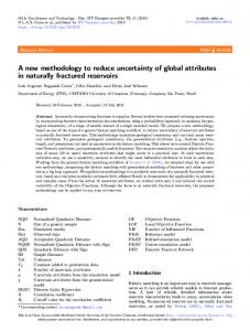
Step 1: select the modelling options and the algorithm of solution. Then, for different values of standard deviation task times, find the layout solution. Task Times are assumed to be distributed according to a one-parameter normal distribution. Different values of the coefficient of variation are equal to 0.1, 0.15, 0.2, 0.25, 0.3, 0.35 and 0.4. Thus seven different layouts are found out. An extra layout solution derives from an additional set of values of standard deviation task times with coefficient of variation uniformly distributed between [0.1, 0.4] (Fig. 1). Step 2: evaluate set1 performance indicators (LEp and BEp ) on the layout solutions. Select solutions that for each different LEp have a higher BEp . This means to select the better-balanced layout for each solution with different design cost (from the most economical to the most expensive) (Fig. 2). Step 3: perform a simulation analysis on these selected solutions, with different values of standard deviation task times, and collect performance indicators (set 2) in order to compare performance and to check solutions stability as regards the uncertainty on standard deviation task times (Fig.3). σ = 0.1 µ σ = 0.15 µ ... σ = 0.4 µ
modelling options: paralleling single mode one sided
…
through simulation in advance to perform step 3, in order to see if SD is a significant input. But an influence of SD on principal output would be probably found, as also verified in the case studied.
CASE STUDIED AND MODEL BUILDING Case studied is an ALB problem in a small enterprise that produces trailers. The problem was referable to a type I ALB, one-sided line, paralleling allowed, cycle time equal to 240 minutes, and total number of tasks equal to 53. Mean times of tasks execution were available from historical registrations, but the entire data-sheet was not on hand. This is a very usual situation when facing with data collection in SME. The heuristic used to find the solution is a modification of Gaither's incremental utilization heuristic [Gaither 1996] proposed in [Mc Mullen and Frazier 1997]. In our application the rule implemented for the assignment of tasks into work-centres selects the task that would result in the highest cell utilization, based on the expected task time. Other rules or heuristics are easily implementable. The heuristic is designed for mixe d-mode production: reducing the stochastic task durations of the mixed-model production demand into composite stochastic task durations turns mixed mode production to an equivalent single mode production. The algorithm also permits paralleling of tasks, allowing multiple workers to exist within cells. The simulation model (build for the step 3 of the methodology) was developed in Java, using Java Simulation package. Each simulated production run for each selected lay-out and each value of SD is replicated 100 times. Simulations were run until steady-state conditions were attained, whereupon outputs were stored. Each run was continued for 120 hours of production. When tasks in a work-centre are not completed within the cycle time, no off-line completion is provided, because of the considerable dimensions of the manufacture. Rather, extended cycle time has been considered. Because there are no buffers between work-centres, this event cause line blocking and idle time of operators. No buffering between station brings the value of WIP to be equal to the number of station in the line.
layout #1 layout #2 … layout #7
σ = U[0.1, 0.4] µ
Algorithm: heuristic
layout #8
Figure 1 Finding the algorithm layout solution for different values of σ (step 1).
LEp
BE p
layout #1
0,7
0,68
layout #2
0,6
0,79
layout #7
0,8
0,8
layout #8
0,7
0,63
layout #1 layout #2
… layout #7
Figure 2 Selecting solutions that for each different LEp have a higher BEp (step 2). σ = 0.1 µ σ = 0.15 µ
σ = U[0.1, 0.4] µ
Step 1 and step 2 of methodology have been performed. Results are shown in Table 1 and Fig. 4. The heuristic finds a lay-out solution with one operator per work-center (paralleling has not been used). Among the eight possible layouts found, only three have different LEp . Remind that different LEp finally means different numbers of workcentres in the line, and thus different design cost. Layout #1 has the higher LEp and the lower number of stations, 7. This layout is selected for the next step as the most economical (and also well balanced). For increasing values of cv, the heuristic found layouts with one more station, 8. For 0.15 ≤ cv ≤ 0.35, the number of stations does not change, resulting in unchanged values
POT, CTR … SIMULATION
... σ = 0.4 µ
RESULTS
POT, CTR … …
1ayout #1
POT, CT R … POT, CTR …
Figure 3 Performances comparison and stability analysis through simulation (step 3). Naturally, an analysis of variance on the selected solutions came out from step 2 could be performed
ISBN: 1-56555-268-7
844
SCSC '03
CTR
of LEp . In this range an increasing value of BEp can be observed. Thus, for the same design cost configuration, the layout #6 is selected as the better balanced. Note that also layout #8, resulting from the heuristic solution with uniform distribution of cv between [0.1, 0.4], has the same number of station, but a lower BEp . Layout #7 is also selected, despite the low value of LEp (one more station in the line). In effect even though this layout has the higher design cost, it has been found for a high value of cv (that means for a high dispersion of task times). Thus, a higher stability with respect to uncertainty of task times SD can be expected. This analysis shows how, in this case, the task times SD is not a much significant model input when searching solutions with different design costs. In effect for a wide range of cv (0.15 - 0.35), solutions have the same number of stations. In this range it is possible to find out the layout with the best balance efficiency (layout #6).
1,3
layout #1 (cv =0,10) layout #6 (cv=0,35) layout #7 (cv=0,40)
1,2 1,1 1,0 0,9 0,8 0,7 0,6 0,10 0,15 0,20 0,25 0,30 0,35 0,40 rdm cv 100% POT 80% 60% 40%
Table 1.
20%
cv
m
LEp
BE p
layout #1
0,10
7
86,6
95,0 selected
layout #2
0,15
8
75,8
76,5
layout #3
0,20
8
75,8
81,9
90%
layout #4
0,25
8
75,8
90,6
85%
layout #5
0,30
8
75,8
93,7
80%
layout #6
0,35
8
75,8
95,9 selected
75%
layout #7
0,40
9
67,4
89,0 selected
70%
layout #8
U[0.1,0.4]
8
75,8
89,3
65%
0% 0,10 0,15 0,20 0,25 0,30 0,35 0,40 rdm 95% UTIL
60% 0,10 0,15 0,20 0,25 0,30 0,35 0,40 rdm
CT = 240 min 340 320 300 280 260 240 220 200 180 160
100% 90% 80% 70% 60%
LEp
50%
BEp
40% 0,10 0,15 0,20 0,25 0,30 0,35 0,40
rdm
0,10 0,15 0,20 0,25 0,30 0,35 0,40 rdm
cv 1900
Figure 4.
1850 1800
Step 3 has then been executed in order to compare layout#6 with the much economical layout #1, and the best performing layout#8. Results are shown in Fig. 5. Graphs outline how performances of each one of the three layouts are influenced by different values of SD task times. This can be meaningful especially for layout #1, because it is a heuristic solution with very little SD task times assumed. In effect it can be observed how layout#1 CTR and actual CT (CT act) are acceptable only for cv
ISBN: 1-56555-268-7
CTact = 1 / TP [min]
AFT [min]
1750 1700 1650 1600 1550 1500 0,10 0,15 0,20 0,25 0,30 0,35 0,40 rdm
Figure 5.
845
SCSC '03
REFERENCES
equal to 0.1, while, for increasing values of cv, the gap from desired values (CTR = 1 and CT act = 240 min) are significant (20% for cv = 0.35). POT is lower than 100% also for cv = 0.1, even though CTR =1; this means that desired values of CTR is achieved only by virtue of overall compensation between anticipation and lateness in task completing. Finally, average system utilization (UTIL) is comparable with that one of layout #6, although the LEp was higher. This signifies that manies line blocking occurs (as POT shows) causing idle time of operators. As expected, layout #7 has the best CTR, POT and TP for any cv. However, layout #6 for cv ≤ 0.25 and cv = U[0.1,0.4] achieves desired value of CTR, but with lower design costs. Better performances of layout #7 with respect to performances of layout #6 can be observed for CTR and AFT. CTR is about 8% higher in #7 than in #6, for each value of cv. AFT is an important indicator in this study, because it impacts directly on time execution of an orders, that was indicated as a critical performance by the enterprise management. AFT maximum gap between the two layouts is about 2% for cv =0.4, and even less for lower values of cv. These better performances have not been considered sufficient to compensate the higher design cost of layout#7. Thus, layout #6 has been chosen as the final solution.
Bruzzone, A., and S. Saetta. 2002. "LESNEX: LEan Simulation Network of Excellence.", HMS2002 and MAS2002 International workshops, (Bergeggi, SV, Italy, October 3-5). Driscoll, J., and D. Thilakawardana. 2001. "The Definition of Assembly Line Balancing Difficulty and Evaluation of Balance Solution Quality.", Robotics and Computer Integrated Manufacturing, 17, 81-86. Gaither N., 1996. Production and Operations Management, 7th ed. Duxbury Press, Boston, MA. Grabau, M.R., R.A. Maurer, D.P. Ott. 1997. "Using Simulation to Generate the Data to Balance an Assembly Line.", in Proceedings of the 1997 Winter Simulation Conference, WSC '97, (Atlanta, GA, December 7-10). 733-738. Kottas, J.F., and H.S. Lau. 1981. "A Stochastic Line Balancing Procedure.", International Journal of Production Research, vol. 19, no. 2, 177-193. Lee, T.O., Y. Kim, Y.K. Kim. 2001. "Two-Sided Assembly Line Balancing to Maximize work Relatedness and Slackness.", Computers and Industrial Engineering, 40, 273-292. Leu, Y., L.A. Matheson, L.P. Rees. 19994 "Assembling Line Balancing using genetic algorithms.", Decision Sciences, 25(4), 581-606. Lyu, J. 1997. "A Single-Run Optimisation Algorithm for Stochastic Assembly Line Balancing Problems.", Journal of Manufacturing Systems, vol. 16, no. 3, 204-210. McMullen, P.R., and G.V. Frazier. 1997. "A Heuristic for Solving Mixed-Model Line Balancing Problems With Stochastic Task Durations and Parallel Stations.", International Journal of Production Economics, 51, 177-190. McMullen, P.R., and G.V. Frazier. 1998. "Using Simulated Annealing to Solve a Multiobjective Assembly Line Balancing Problem With Parallel Workstations", International Journal of Production Research, vol. 36, no.10, 2717-2741. Peterson, C. 1993. "A Tabu Search Procedure for the Simple Assembly Line Balancing Problem.", in Proceedings of the Decision Sciences Institute Conference, (Whashington, DC,). 1502-1504. Sarin, S.C., E. Erel, E.M. Dar-El. 1999. "A Methodology for Solving Single-Model, Stochastic Assembly Line Balancing Problem.", Omega: International Journal of Management Sciences, 27, 525-535. Silverman, F.N, and J.C. Carter. 1986. "A Cost-Based Methodology for Stochastic Line Balancing With Intermittent Line Stoppages", Management Science, 32 (4), 455-463. Suresh, G., and S. Sahu. 1994. "Stochastic Assembly Line Balancing Using Simulated Annealing.", International Journal of Production Research, vol. 32, no. 8, 18011810.
CONCLUSIONS A methodology for approaching the ALB problem with the minimum of data collection has been proposed. The method allows using algorithms (in our cases heuristics) that consider stochastic task times, without having standard deviation of task times on hand. The procedure proved to be easily and quickly implementable, thus reducing as much as possible the costs of the simulation study. This allowed to apply the method to a small enterprise that produces trailer. In the case studied, results show how task times standard deviation is an input that does not have a relevant influence on the design costs of the solution found. Uncertainty on the system performances is quantifiable and acceptable for the type of application, and usable outputs for the choice of the best solution have been obtained. Further developments of the proposed methodology will consist in the implementation of different solution-finder algorithms, based on different techniques such as simulation annealing, tabu search and genetic algorithms. This will allow studying the standard deviation influence on solutions generated from different methods. Moreover the simulation model developed in Java will be improved and made more flexible in order to achieve the direct applicability to a wider range of real applications. This will result in a contraction of model building time, making this methodology very useful where Lean Simulation approach is required.
ISBN: 1-56555-268-7
846
SCSC '03