such as cost or dependability. Design space exploration often appears as a challenging problem in application areas, such as dependable embedded systems ...
A Model-driven Framework for Guided Design Space Exploration ´ ´ Abel Heged¨us, Akos Horv´ath, Istv´an R´ath and D´aniel Varr´o Department of Measurement and Information Systems Budapest University of Technology and Economics Budapest, Hungary Email: {hegedusa,ahorvath,rath,varro}@mit.bme.hu
Abstract—Design space exploration (DSE) aims at searching through various models representing different design candidates to support activities like configuration design of critical systems or automated maintenance of IT systems. In modeldriven engineering, DSE is applied to find instance models that are (i) reachable from an initial model with a sequence of transformation rules and (ii) satisfy a set of structural and numerical constraints. Since exhaustive exploration of the design space is infeasible for large models, the traversal is often guided by hints, derived by system analysis, to prioritize the next states to traverse (selection criteria) and to avoid searching unpromising states (cut-off criteria). In this paper, we define an exploration approach where selection and cut-off criteria are defined using dependency analysis of transformation rules and an algebraic abstraction. The approach is evaluated against other exploration techniques and illustrated on a cloud infrastructure configuration problem. Index Terms—design space exploration; model transformation;
I. I NTRODUCTION Design space exploration (DSE) is a process to analyze several “functionally equivalent” implementation alternatives, which meets all design constraints in order to identify the most suitable design choice (solution) based on quality metrics such as cost or dependability. Design space exploration often appears as a challenging problem in application areas, such as dependable embedded systems [1], [2] and IT system management, where model-driven engineering (MDE) techniques are already popular. DSE can be performed either during the design process to find optimal designs or during runtime to help dynamic reconfigurations. In traditional DSE problems, the design constraints and quality metrics are numeric attributes to express cost, time or memory limits, etc. However, systems with modular software and hardware architectures (like AUTOSAR [3] in the automotive domain or large reconfigurable architectures) introduced complex structural constraints that express restrictions on the graph-based model of the system under design. These constraints may include restrictions related to the communication architecture or allocation of software and hardware resources. Furthermore, during the design of dynamically changing systems (e.g. reconfiguration of virtual servers over physical ones), the design space exploration also requires the dynamic creation and deletion of elements.
Existing DSE approaches usually apply model checking with exhaustive state space exploration or solve finite domain constraint satisfaction problems that cannot effectively handle structural constraints and dynamic manipulation of elements. In order to alleviate these issues, designers often provide additional information (hints) about the system (e.g. from earlier experience or by some analysis) that can reduce the design space to a more feasible size [1]. The design process is often complemented with different design and analysis and verification tools, which can also provide (mathematically well-founded) hints about the model in the early stages of development. These hints may express additional system properties, which can be incorporated in the DSE process to assist the evaluation of alternate solutions. Guided model-driven design space exploration aims to explore alternative system designs efficiently by making use of advanced model-driven techniques (e.g. incremental model transformations) and hints (obtained by analysis tools or provided by the designer). These hints are interpreted during the exploration to continue along promising search paths (using selection criteria) and to avoid the traversal of unpromising designs (by cut-off criteria). Additionally, the use of incremental techniques leads to exploration strategies that are able to find additional (alternative) solutions, which are close to an earlier solution. In our paper, we propose a model-driven framework for guided design space exploration, where the system states are graphs, operations are defined as graph transformation rules, while goals and constraints are defined as graph patterns. We extend our previous work on model-driven design space exploration [4] by incorporating hints during the exploration strategy, which are derived from dependency analysis of transformation rules and algebraic analysis on the Petri net abstraction of the system [5]. Cut-off and selection criteria are defined based on these hints [6], and their evaluation guides the design space exploration by identifying dead end states and prioritizing possible operations, respectively. Major contributions of this paper with respect to our previous work [4], [6] are (i) the design and implementation of a complete model-driven framework for guided design space exploration, (ii) a guided exploration strategy that exploits various hints and (iii) an experimental evaluation of the approach on relevant case studies.
II. OVERVIEW OF THE A PPROACH In our paper, we describe a novel framework that combines the model-driven approach of design space exploration (DSE) with guided exploration techniques building on hints from analysis and guidance through cut-off and selection criteria. The schematic overview of the framework for guided design space exploration is illustrated in Figure 1.
Fig. 1.
Model-driven Guided Design Space Exploration
First, the design problem description specifies the domain where the exploration takes place to produce solutions. It includes: (1) the initial state of the system at the start of the exploration, (2) the set of manipulation operations (called labeling or exploration rules) defined on the system, (3) goals described as structural or numerical constraints, which need to be satisfied by solution states found by the exploration, and (4) global constraints, which are satisfied by the initial and solution states and all intermediate states on the trajectory between them. The detailed discussion of the problem description is found in Section IV The design space exploration performs the search for solutions by exploring the design (or state) space of the problem description. It starts from the initial state and traverses reachable states by applying the operations on the system (see Section III). In order to find a solution quickly exploration is often aided by an exploration strategy (detailed in Section VII). A simple strategy (as proposed in [4]) may use random selection in a depth first search or statically assign priority levels to operations. However, a more advanced strategy should also determine whether a given state will never lead to a valid solution (i.e. it is a dead end) and states reachable from it should not be traversed. In a guided approach, the exploration strategy relies on guidance, which uses hints for driving the traversal and identifying dead ends. Hints are information originating from the designer or (as in our paper) from some automated analysis carried out using formal methods that often abstract the design problem description. The result of the analysis can be information regarding the number of operation applications (called as an occurrence vector), partial ordering of operations, restricting
the set of required operations etc. These results are often generated before the exploration in a preprocessing phase. Our guided approach uses occurrence vectors and dependency relations between rules as hints (see Section V). Finally, the guidance calculates and interprets hints and provides decision support for the exploration strategy (see details in Section VI). In our approach, guidance is defined as the evaluation of cut-off and selection criteria based on the current state and the hints (as defined in [6]). Cut-off criteria identify dead end states and bound the exploration, while selection criteria prioritize available rules in a state by their likelihood of leading to a final (solution) state. Challenges of Guided Design Space Exploration: While existing model-driven frameworks (e.g. GROOVE [7]) are able to explore the design space of smaller problems by exhaustively traversing reachable states and checking global constraints and goals in each state, they use no global information when selecting the applied labeling rules. Our guided approach, however, takes advantage of hints and guidance that help the exploration and addresses the following challenges: • identify decisions in the exploration: the framework should clearly separate the guidance from the exploration strategy to easily allow the modification of both parts of the framework. • soundly reduce traversed design space: the guidance should reduce the number of traversed states before finding solutions, but it must ensure that no valid solutions are removed by the cut-off criteria. • provide optimal solutions: the guided framework should find the solutions that are optimal (with respect to a user-defined metric). Moreover, the framework should be able to continue exploration to find other (less optimal) solutions if necessary. • extensibility: the approach should be easily applicable on different design problems and the set of criteria should be extensible. This is a key feature for adapting the framework to various domains. III. G UIDED D ESIGN S PACE E XPLORATION The guided design space exploration approach is based on a general search process, which traverses the design space starting from the initial state. This general process includes a step (Evaluate criteria), which relies on the guidance and hints provided by system analysis to the different exploration strategies (identify decisions challenge). The search process, depicted in Figure 2, consists of the following steps: 1) Check operation applicability. First, labeling rules (of the design problem description) are checked for executability (i.e. whether they can be executed in the current state of the model) and this information is passed to the criteria evaluation. 2) Evaluate criteria. The cut-off and selection criteria are evaluated using the hints (the rule dependencies and the occurrence vector) and the results are stored. 3) Cut-off? If at least one of the cut-off criteria were satisfied during the evaluation, or there are no applicable
In order to provide an appropriate infrastructure for clients, the configuration of the cloud infrastructure must meet certain requirements (including complex structural constraints), e.g. an application and a storage subsystem is required for a cloudbased web service. Such an infrastructure is shown in Figure 3.
Fig. 2.
Workflow of the guided design space exploration Fig. 3.
4) 5) 6)
7)
8)
rules, the state is a dead end and the branch is cut. Select rule. The design space exploration then selects the next applicable rule based on the evaluation results. Apply rule. The selected rule is applied to the model resulting in a new model state. Check new state. The global constraints and goals are checked on the new state to decide whether it is an invalid or solution state. a) Is valid state? If any of the constraint are violated, the state is invalid and the exploration continues from the previous state. Note, that a state is also considered invalid if the exploration has visited it earlier, since in this case the reachable states are already explored from this state. b) Is solution found? If all of the goals are satisfied, the state is a solution. Save solution. When a solution model is found, the trajectory (with the executed rules and corresponding model state information) is saved to a solution list. Continue search. Once the new model state is checked, the next applicable rule is selected from a valid new state, otherwise from the previous state.
Design space exploration terminates either once a predefined number of solutions are found (or if the found solution is acceptable by other, user-defined metrics) or if there are no applicable rules within the limited search space. Since a hint does not always represent a feasible trajectory, the exploration is restarted with an alternative vector if more solutions are required to be found. IV. D ESIGN P ROBLEM D ESCRIPTION A. Motivating Example: Cloud Configuration Today services are often built on top of a cloud middleware (CM) using components as building blocks to be able to scale dynamically to meet demands. Servers (S) and highavailability clusters (Cl) can be deployed on the cloud middleware, while databases (DB) are installed on servers and applications (App) are executed over databases. Finally, servers can also be deployed on clusters and storage (St) subsystems can only operate over clustered servers.
An example system providing reliable service
To satisfy this constraint the cloud configuration has to be designed in an appropriate way. We assume that regular change management commands (including deletion or creation, e.g. deploying a new database) are issued by some middleware service broker. If the current infrastructure of the cloud detects that the required parameters cannot be satisfied by the actual cloud configuration, reconfiguration operations are to be initiated, which lead the system into a state where all constraints are met. To deal with changes of requirements and possible commands, guided design space exploration is used to find command sequences that should be executed to create a valid configuration. B. Initial State States are represented as instance models that conform to a metamodel. This metamodel describes the problem domain and the initial state defines where the design space exploration starts from. A metamodel M M for a design problem includes the set of model element types of the domain, their attributes and relationships between model elements. An instance model is a model that conforms to a metamodel, if it only includes model elements and relations with types defined in M M .
Fig. 4.
Metamodel and instance model of the cloud infrastructure
The left part of Figure 4 shows the metamodel for the cloud case study. The metamodel contains a cloud component Node designated graphically as a rectangle. The specific components Socket, Server, Database, Application and Storage are specialized from this node, Socket is a generalization of Cloud MW and Cluster ). Edge deployedOn is a relation that connects two different components denoting that the source node is deployed on the target node of this relation. The right part of Figure 4 illustrates an instance model containing a
Fig. 5.
Example goal and global constraint
database d deployed on two servers s1, s2 that are on cloud c. Note that in the rest of the paper, we omit deployedOn (dOn) relations by illustrating the relation using vertical arrangement of components. C. Goals and Global Constraints Goals and global constraints of the design problem description are defined as bounds on the number of matches for graph patterns. Graph patterns represent conditions that have to be fulfilled by a part of the model, this part is called a match. The left part of Figure 5 shows an example goal, which specifies that a solution model includes at least 5 databases deployed on clusters, while the right part shows a global constraint, that allows maximum 100 servers deployed on clouds altogether. D. Labeling Rules The labeling rules that define the possible manipulation operations on the problem state are represented by graph transformation (GT) rules. GT rules [8] are specified by a precondition (or left-hand side - LHS) pattern determining the applicability of the rule and a postcondition (or right-hand side - RHS) pattern that specifies the result model declaratively. The negative application conditions (NAC) of a GT rule specify patterns that prohibit the application of the rule if they have matches. The reconfiguration actions of the ongoing example is captured by a set of graph transformation rules in Figure 6. An overview on using graph transformations for software architecture reconfigurations can be found in [9].
however, a Cl cannot have more than two S deployed on it. Rule addCl produces a new Cl deploying it on top of a CM , addDb adds a new database DB deploying it on top of two S that have no other Node deployed on them, addApp creates a new application App deploying it on top of two DB that have no other Node deployed on them. Finally, addSt adds a new storage St deploying it on two S that are deployed on the same Cl and have no other Node deployed on them. It is important that the set of goals, constraints and rules are easily extensible by the designer (extensibility challenge). The design problem description is not hard-coded into the exploration and can be modified using a high-level textual language [10]. Our framework also supports dynamic handling of goals, constraints and rules, e.g. to generate solutions for different subsets of rules. Application of a Rule: r alters the model by replacing the pattern defined by LHS with the pattern of the RHS (illustrated in Figure 7). This is performed by (1) finding a match of the LHS in the model (2) checking the negative application conditions, (3) removing a part of the model that can be mapped to the LHS but not the RHS yielding an intermediate graph and (4) adding new elements to the intermediate graph, which exist in the RHS but not in LHS or updating existing elements, yielding the derived graph. E. Design Space The design space traversed by the guided exploration approach is represented by a graph transition system containing the states, which are reachable from the initial state by applying the labeling rules. A graph transformation sequence (GT sequence) is a sequence of GT steps (application of a rule on a given match), i.e., a sequence of rule applications. A graph transition system GT S is defined as a graph where nodes are instance models, and edges are rule applications. Starting from G0 (initial state) the state space (i.e. the reachable instance graphs) of GT S is represented by executing all applicable rules from a given initial graph as long as possible. The different matches of applicable rules may lead to different edges in GT S. A path in the graph transition system is a GT sequence also called a trajectory between two states. A state Gi is reachable from G0 iff there is a trajectory in GT S from G0 to Gi . In Figure 7 an extract of the graph transition system of the running example is shown. On the left, the root of the graph transition system is the start graph G0 where the system configuration contains a CM , three S , and one DB components. Rules addS , addCl , and addCM are applicable to G0 , here we follow the application of addS and addCl . V. H INTS
Fig. 6.
Graph transformation rules
The addCM rule adds a new cloud CM , addS creates a new server S deploying it on top of a CM or cluster Cl ,
The design space exploration framework uses graph transformation sequences to reach solution states. In order to guide the exploration efficiently, both the amount and order of rule applications are useful hints.
of times that rule ri is applied during the execution. During the design space exploration, the number of times rule ri has been applied in a given path is stored in the application vector (v a ) as v a (i). An execution path of the state space exploration is compliant with σ if v a ≤ σ (the number of applications is less or equal for each rule). Throughout the paper we use the difference σ(i) − v a (i) as the remaining application number #i of rule ri . This number is stored as an attribute for nodes in Gd (see Figure 8) together with the state of ri that is either enabled or disabled in a given state. C. Using Dependency Graph in Design Space Exploration
Fig. 7.
A part of a graph transition system
A. Graph Transformation Rule Dependency Given the precondition-postcondition nature of GT rules, it is possible to derive which rules might be affected by the application of a given rule. For example, the application of a GT rule r can alter the model in a way that other rules, which were disabled before, become enabled (or the other way around), thus the application of these rules depend on the application of r. The dependencies between rules are independent of the instance models, and can be derived from the rule definitions. This analysis can be carried out using various techniques, such as critical pair analysis [11] or conditional transformation-based dependency analysis [12], and results in a matrix of dependencies between rules.
The model state and the dependency graph are tightly connected for a given initial graph and occurrence vector. Figure 9 illustrates how the application of a GT rule affects the current state and the remaining application number. First, the current state is depicted as the model M (representing the current cloud configuration) and remaining application number and state of each node in the dependency graph Gd (in short, the current dependency graph). The color of the nodes (e.g. naddS ) of Gd represent the state of the corresponding GT rules (raddS ), green (dark) background for enabled, grey (light) for disabled. The number near each node is the remaining application number (e.g. #addS = 3).
Fig. 9. Fig. 8.
Dependency graph example
The result of the analysis is used to create a dependency graph (Gd , illustrated in Figure 8) of the rules, where an arc denotes sequential dependency (i.e. the application of the source rule may affect the match set of target rule). Note that there may be arcs in both direction between two rules. As illustrated on Figure 8, rule addS depends on rules addCM, addCl , while rules addSt, addDB depend on addS (the sets are represented by J raddS and raddS I, respectively). B. Transformation Rule Occurrence Vector We use a Petri net abstraction technique introduced for GTS in [13], which provides hints that estimate how many times each rule is applied in order to reach a given state. A candidate occurrence vector (σ) is a solution of the analysis of the Petri net abstraction, where σ(i) is the number
GT rule application and its effects on the dependency graph
In the course of design space exploration, the next GT rule, which is applied (raddS in the example) is selected from the set of enabled rules. The application has the following effects on the models: (a) model M changes according to the rule definition (here, a new server S is added to cloud CM ), the new model is illustrated as M 0 (b) the #addS is modified to represent that the rule is applied (it decreases from 3 to 2) (c) Gd is also changed to G0d , as #addS decreased and the applicability of GT rules may change (here raddDB becomes enabled). The design space exploration then continues from M 0 by selecting a rule based on G0d . VI. G UIDANCE A. Overview of Cut-off and Selection Criteria Cut-off and selection criteria are used as guidance to decide in which order the states of the design space are explored.
We define formal criteria over the current dependency graph, which are evaluated to support decisions: • Cut-off criteria inspect the current dependency graph and return a boolean result, which is true if further exploration of the current branch cannot lead to a goal state with a compliant trajectory. In this case, the exploration continues from an other state instead of executing a rule in the current state. • Selection criteria take the current dependency graph and define an ordering of applicable rules. A given rule ri is placed before an other rule rj , if the execution of ri is more promising, based on the criteria and the current state, than the execution of rj . B. Criteria for Guided Design Space Exploration We used the following cut-off and selection criteria, which are meaningful when dealing with guided DSE. • Non-compliant path (Look-ahead) cut-off criterion. If the application of any GT rule would make the current execution path non-compliant with the occurrence vector, it can be cut. • Permanently disabled rule cut-off criterion. The current path can be cut if there is a disabled rule, which still has to be applied based on the occurrence vector, but rules that may enable it will not be applied. • Independent rule application selection criterion. Applicable rules with no forward dependency should be applied as early as possible to reduce the number of different applicable operations later in the trajectory. • Maximal forward-dependant application path selection criterion. Among the applicable rules at any given state of the exploration, the rule that affects more applications should be applied earlier in the trajectory. C. Criteria Evaluation The criteria defined over the dependency graph are evaluated at every state using an algorithm described in [6] (interpret hints challenge). The main steps of the algorithm are: (1) a starting point is selected from the criterion, (2) the list of nodes satisfying the starting point are created, (3) the operations of the criterion are applied on each node and (4) the result is assembled as a boolean value (cut-off criteria) or an ordered list of rules (selection criteria). VII. E XPLORATION S TRATEGY Guided exploration strategies can be categorized by the used hints and guidance. We specified two guided strategies (see Figure 10), the first uses occurrence vectors only as hints (occurrence), while the other uses rule dependency as well (full guidance). Note that the full guidance strategy uses rule priorities only if two labeling rules were evaluated as equal by the guidance. These strategies are compared to the fixed priority depth-first search strategy. Figure 11 illustrates the design space exploration for these techniques on a simple example. The circles denote the traversed states which are numbered according to the traversal
Fig. 10.
Comparison of exploration strategies by used hints
order, while the applicable rules are listed beside them. Downward arrows illustrate rule applications, while upward (and dotted) arrows represent backtracking from invalid or cut-off states. The same rule can be applied multiple times at a given state if more than one applicable match is found in the graph (see state 2 on the right side). The exploration terminates when an optimal solution is found. A solution is optimal if the path leading to it contains the least number of rule applications (i.e. it is the shortest trajectory to a solution model). Note that the framework is extensible also to labeling rules with costs and optimal solutions identified by the lowest total cost [5].
Fig. 11.
Comparison of exploration strategies
In the case of the fixed priority strategy, the next applied operation is the one with the highest priority among the applicable ones. In the example, first r1 is applied then r2 . From state 2, first r1 is applied leading to state 3 without applicable rules. After backtracking, r3 is applied instead. Note that after this point all reachable states from state 2 and state 1 are explored before trying r2 in state 0 (which finally leads to an optimal solution). Moreover, as the depthfirst technique is used in the fixed priority exploration strategy, the first solution found by that strategy is often several times longer than the optimal, suboptimal solutions are used as depth limits to force the exploration to find shorter solutions. The occurrence strategy applies operations based on the occurrence vector provided by the system analysis. The example in Figure 11 shows that r2 should be applied twice and r3 once. Therefore, r1 is not applied in state 0 or 2 (highlighted) in order to be compliant to the occurrence vector. In states 3 and 4, the exploration backtracks (as no more rule applications are allowed by the vector) and then continues to find the solution in state 6. The full guidance exploration strategy (illustrated in the right side of Figure 11) takes the dependency relations be-
tween rules into account in addition to the occurrence vector. Therefore, in state 1 (highlighted) it selects r3 for the next application. Rule r2 is applicable on two matches in state 2, the first leading to a dead-end state, while the second application leads to a solution in state 4. Note that the selection in state 1 leads to a reduced traversed design space compared to the occurrence exploration strategy (reduce traversed design space challenge). VIII. I MPLEMENTATION D ETAILS Figure 12 gives an overview of the implemented guided design space exploration framework. The implementation uses the V IATRA 2 model transformation framework [14], which provides metamodeling capabilities and supports model transformations based on the concepts of graph transformations and abstract state machines. Its incremental pattern matcher is used as a powerful query engine [15].
Fig. 12.
Overview of the guided DSE framework
The design space exploration is performed by the constraint satisfaction engine, CSP(M), presented in [4], where rules, goals and constraints (specified using graph transformation rules and patterns) are used in solving constraint satisfaction problems over the input model (both included in the design problem description). The abstraction of graph transformation rules into Petri nets (PN ) and ILP problems are also automated. We used the industry leading IBM CPLEX 1 optimization tool, which supports the calculation of alternate solutions (occurrence vectors used for initializing the dependency graph). The edges of Gd are computed from the transformation rules using the Condor 2 dependency analyzer tool, while the graph itself is built and stored as an EMF instance model. The criteria definitions and the criteria evaluation algorithm (guidance) are implemented in Java as separate components, and are connected to the guided design space exploration strategy . IX. E VALUATION OF THE A PPROACH The aim of the evaluation is to demonstrate that the full guidance strategy is more efficient than the other strategies (namely, fixed priority and occurrence, which we used for 1 http://www.ibm.com/software/integration/optimization/cplex-optimizer/ 2 http://roots.iai.uni-bonn.de/research/condor/
previous measurements in [4]) as it traverses considerably fewer states and does not introduce significant overhead, thus provides better runtime in most cases than the other approaches. The reader is directed to [4] for comparison with other tools (e.g. SICStus Prolog CLP(FD), KORAT and GROOVE), which is omitted here for space considerations. A. Cases used in the Evaluation For evaluation, we used the cloud case study presented in Section IV-A and a service configuration case study (presented in [5]). These cases are relevant in the context of modeldriven DSE as they represent both design time and runtime exploration problems, respectively, and it allows comparison with previous results [4], [5]. Both case studies included multiple cases (see Figure 13). PowerOn cases deal with empty initial models, while Reconfigure cases deal with existing models which must be modified to satisfy goals. In the cloud cases, the goals describe the number of required components (e.g. 2 applications and 2 storage in PowerOn Small ). Furthermore, global constraints are raised to give some limit to the priority based strategy (e.g. a cloud middleware should have at most 100 nodes installed). Finally, the Clustered Database case requires databases to be deployed on clusters (see Figure 5). In the service configuration cases, the models represent a set of services that are reconfigured runtime (e.g. removing faulty or starting new instances) to meet some QoS requirements. The constraints in these cases define the maximum number of services, while goals describe the number of active services and that faulty services are removed. The size of the models are given after the name of the problem, in the cloud cases the required applications and storages subsystems, while in the service cases the maximum number of services, faulty and active services in the initial model and active services in solutions. B. Evaluation Environment and Method The evaluation was carried out 5 times for each test case and strategy in the following way3 : (1) the initial model is loaded into V IATRA 2, (2) the goals, constraints and operations are added to the framework, (3) the exploration component is initialized and runtime measurement is started (using wall time with OS-level nanotime precision). Next, (4) the design space exploration framework looks for an optimal solution. Finally, (5) the runtime measurement is stopped and the results are saved. The exploration is limited to 1 million visited states. C. Evaluation of Results The table in Figure 13 shows the results of measurements using the case study models. For each case, we measured the average length of the shortest discovered solution trajectory (the number of applied rules), the average number of visited states during the design space exploration and the average runtime of the exploration. 3 For measurements we used a computer with Intel Centrino Duo 1.66 GHz, 3 GB memory, Win7 Prof. 32 bit, Eclipse 3.6.1, V IATRA 2 3.2
Fig. 14.
•
Fig. 13. Results for exploration until optimal solution († denote cases where exploration did not terminate in all tests)
• •
We made the following observations based on the results from the different cases: Find optimal solution: We observed that the usage of occurrence vectors as hints in the exploration ensures that the first solution found by such strategies is optimal as well (optimal solutions challenge). In our observations, the fixed priority strategy, finds longer solutions first and traverses a large number of states even in case 4 (which is the smallest), before finding an optimal solution. Low overhead of criteria evaluation: The evaluation of cut-off and selection criteria is performed at every new traversed state, and it might (in principle) slow down the exploration considerably. However, our observation is that criteria evaluation has very low overhead (less than 5% of the overall runtime). The full guidance strategy requires some initial bookkeeping (building dependency graph and initializing criteria), but afterwards, it traverses 1000 states in roughly 600ms (similarly to the other strategies). Rule dependency increases efficiency: In all cases, the full guidance strategy traverses significantly fewer states than the occurrence strategy. Note that the only case when the fixed priority strategy traverses less states is case 6, where the occurrence vector is recalculated at least 20 times before finding a feasible solution. It is important to note that in these cases, the full guidance approach outperforms the occurrence strategy by identifying infeasible occurrence vectors with less exploration. Figure 14 illustrates how the number of traversed states for these two strategies when exploring infeasible occurrence vectors in case 5. The graph clearly shows that the full guidance strategy explores only half the states in average that the occurrence does. Note that in case 2, the occurrence strategy did not find a solution inside the limit in some instances. To sum up the results of the evaluation, we observed that:
Reduction in visited states by the full guidance strategy
The combined use of occurrence vectors and rule dependency for cut-off and selection criteria based guidance outperforms our previously published strategies. The added computation required for criteria evaluation does not significantly increase runtime. The under-approximation of the occurrence vector based analysis ensures that guided exploration strategies always find optimal solutions first.
D. Limitations Our guided DSE relies on the quality of the hints provided for the design problems. This manifests as a limitation in the following cases: (1) if the occurrence vector is infeasible and it includes a large number of rule applications (similarly to case 6) and (2) if the dependency graph (Gd ) is close to a complete directed graph, which makes criteria less effective as guidance. Finally, a large Gd (in case of large set of operations) may increase the overhead of criteria evaluation. X. R ELATED W ORK Model-driven guided design space exploration implemented over graph transformations is a novel idea in the field, however, similar approaches are not unprecedented in a broader research scope as described below. In our previous work, [5] introduces the usage of occurrence vectors for hints in the optimization of GT systems, while [6] defines the dependency graph and the evaluation algorithm for arbitrary cut-off and selection criteria. Finally, [4] describes the formal foundations of model-driven DSE used in our approach. While we apply these techniques, the design of the guided DSE framework and guided exploration strategies are major novel contributions. Graph Transformation based Approaches: The approach in [16] is similar to our approach as it also exploits the dependencies between GT rules using critical pair analysis. Here, GT systems are enhanced with control flow as well and the dependency information helps in discovering possible runtime problems. Model checking approaches to analyze GT systems are similar to our approach as they also perform state space exploration. One can categorize them as compiled approaches such as [17]–[21], which translate graphs and GT
rules into off-the-shelf model checkers to carry out verification, and interpreted approaches like [7], [22], [23], which store system states as graphs and directly apply transformation rules to explore the state space, similarly to our approach. They place emphasis on exhaustive traversal (e.g. by optimizing the storage of individual states), while we aim at finding solutions quickly using guidance and hints. Model-driven Design Space Exploration Techniques: The DESERT tool suite [24] provides model synthesis and constraint-based DSE for DSMLs with structural semantics using ordered binary decision diagrams for encoding and pruning the design space. [25] presents a generic DSE framework extending upon DESERT by supporting arbitrary analysis tools and includes model transformations for mapping design problems to intermediate and low-level formats. The OCTOPUS Toolset [26] uses an intermediate representation for design problem specification and performs DSE using integrated analysis tools. These are all compiled approaches, where the design problems are specified as models and model transformations are applied to derive inputs for analysis tools. Furthermore, the analysis tools perform the DSE, while in our approach, they only provide hints for the exploration. Sch¨atz et al. [27] developed an interactive, incremental process using declarative transformation rules for driving the exploration. The rules are modified interactively to improve DSE performance, which can be considered as a guidance. However, the hints do not originate from analysis, contrary to our approach. Guided Design Space Exploration Techniques: Existing DSE techniques sometimes use guidance information to reduce the number of alternatives that are evaluated. Mohanty et al. [1] use “human in the loop” guidance in addition to symbolic search techniques for finding candidates, which are then analyzed using low-level simulation to find the final design. In [2], different chip design alternatives are evaluated using implementation specific information from earlier designs (e.g. cycle counts and energy consumption) or estimates by experienced designers. The hints are a collection of values, while guidance is used for selecting optimal mappings. These approaches use hints and guidance for reducing the design space, although hints originate from earlier experience or human interaction instead of formal mathematical analysis of the design problem. Structural Constraint Solving: Structural constraint solving aims to find object graphs that satisfy given constraints both on attributes and (object) structures by exploring a (usually) bounded number of possible object graphs. The CUTE [28] framework uses a combination of symbolic and concrete execution to derive path constraints for each separate execution paths. Java PathFinder [29] is based on Generalized Symbolic Execution that first introduced the use of model checkers for solving structural constraints. KORAT [30] performs specification based testing by using a predicate representing the properties (constraints) of the
desired output structures and explores the input state space of the predicate using bounded exhaustive testing. In all of these approaches hints are given in the form of explicit bounds on the size of the state space. However, they cannot restrict how solutions are achieved from the initial model, meaning that no constraints can be defined to hold on states visited during a solution trajectory. In our case it is supported by global constraints and explicit rule definitions, thus resulting in fundamentally different search strategies. Metaheuristic based Search Strategies: There are several single-solution based metaheuristic techniques used in search based software engineering for the optimization of various design space exploration problems [31]. Guided local search based techniques [32] uses a predefined schema to inject penalties into their guidance functions.Simulated annealing based techniques [33] are similar to hill climbing approaches with the ability to avoid local optimum solutions by permitting moves to less fit states, with a decreasing probability over time. Common in these techniques that they use an iterative traversal algorithms to improve candidate solutions with regards to their measure of quality (e.g., guidance function). However, with no hints available about the global optimum these techniques rely only on neighboring states when selecting the next step on the contrary our approach uses hints like the occurrence vector for finding the optimum solution. XI. C ONCLUSION AND F UTURE W ORK Guided DSE exploration uses hints to reduce the number of states traversed when searching for solutions. Hints are used (i) to identify dead-end states (cut-off criteria) and (ii) to order applicable rules in a given state (selection criteria). In the current paper, we defined a model-driven framework for guided DSE, which uses rule dependency and occurrence vectors as hints for the exploration strategy. Evaluation of the exploration strategies using a cloud configuration problem showed that our criteria-driven approach can reduce the design space further thus increasing the efficiency of the exploration. Future work. We plan to improve the framework by better reusing the design space when exploring subsequent occurrence vectors to identify states where the traversal should continue. We are also working on defining problem-specific criteria and specialized algorithms to increase the efficiency of the approach. ACKNOWLEDGMENT This work was partially supported by the SecureChange (ICT-FET-231101) FP7 project, the CERTIMOT (ERC HU09-1-2010-0003) project and additionally, the Janos Bolyai Scholarship. R EFERENCES [1] S. Mohanty, V. K. Prasanna, S. Neema, and J. Davis, “Rapid design space exploration of heterogeneous embedded systems using symbolic search and multi-granular simulation,” SIGPLAN Not., vol. 37, pp. 18– 27, 2002.
[2] B. Ristau, T. Limberg, and G. Fettweis, “A mapping framework for guided design space exploration of heterogeneous mp-socs,” in Proc. of the conf. on Design, automation and test in Europe, ser. DATE ’08. ACM, 2008. [3] AUTOSAR Consortium, The AUTOSAR Standard., http://www.autosar. org/. ´ Horv´ath and D. Varr´o, “Dynamic constraint satisfaction problems [4] A. over models,” Software and Systems Modeling, 2011, 10.1007/s10270010-0185-5. [5] S. Varr´o-Gyapay and D. Varr´o, “Optimization in Graph Transformation Systems Using Petri Net Based Techniques,” ECEASST, vol. 2, 2006, Proc. of PNGT ’06. ´ Heged¨us, A. ´ Horv´ath, and D. Varr´o, “Towards guided trajectory [6] A. exploration of graph transformation systems,” ECEASST, vol. 40, 2010, Proc. of PNGT ’10. [7] A. Rensink, “The GROOVE simulator: A tool for state space generation,” in Applications of Graph Transformations with Industrial Relevance (AGTIVE), ser. LNCS. Springer, 2004. [8] H. Ehrig, G. Engels, H.-J. Kreowski, and G. Rozenberg, Eds., Handbook on Graph Grammars and Computing by Graph Transformation. World Scientific, 1999, vol. 2: Applications, Languages and Tools. [9] L. Baresi, R. Heckel, S. Th¨one, and D. Varr´o, “Style-based modeling and refinement of service-oriented architectures,” Journal of Software and Systems Modelling, vol. 5, 2006. [10] D. Varr´o and A. Balogh, “The model transformation language of the VIATRA2 framework,” Science of Computer Programming, vol. 68, no. 3, pp. 214–234, October 2007. [11] R. Heckel, J. M. K¨uster, and G. Taentzer, “Confluence of Typed Attributed Graph Transformation Systems,” in Proc. ICGT 2002. LNCS. Springer, 2002. [12] T. Mens, G. Kniesel, and O. Runge, “Transformation dependency analysis - a comparison of two approaches,” in Langages et Mod`eles a` Objets (LMO 2006), 2006. [13] D. Varr´o, S. Varr´o-Gyapay, H. Ehrig, U. Prange, and G. Taentzer, “Termination analysis of model transformations by petri nets.” in Proc. ICGT 2006, ser. LNCS, vol. 4178. Brazil: Springer, 2006. [14] “V IATRA 2 Model Transformation Framework, An Eclipse GMT Subproject,” http://www.eclipse.org/gmt/VIATRA2/. ´ Horv´ath, G. Bergmann, I. R´ath, and D. Varr´o, “Experimental as[15] A. sessment of combining pattern matching strategies with VIATRA2,” International Journal on Software Tools for Technology Transfer (STTT), vol. 12, pp. 211–230, 2010. [16] C. Ermel, J. Gall, L. Lambers, and G. Taentzer, “Modeling with plausibility checking: Inspecting favorable and critical signs for consistency between control flow and functional behavior,” in Proc. FASE ’11. Springer, 2011, LNCS 6603. ´ Schmidt and D. Varr´o, “CheckVML: A tool for model checking [17] A. visual modeling languages,” in Proc. UML 2003, ser. LNCS, vol. 2863. Springer, 2003.
[18] S. Edelkamp, S. Jabbar, and A. Lluch-Lafuente, “Heuristic search for the analysis of graph transition systems.” in Proc. ICGT 2006, ser. LNCS, vol. 4178. Springer, 2006. [19] L. Baresi, V. Rafe, A. T. Rahmani, and P. Spoletini, “An efficient solution for model checking graph transformation systems,” ENTCS, vol. 213, 2008. [20] O. M. dos Santos, F. L. Dotti, and L. Ribeiro, “Verifying object-based graph grammars.” ENTCS, vol. 109, pp. 125–136, 2004. [21] L. Baresi and P. Spoletini, “On the Use of Alloy to Analyze Graph Transformation Systems,” in Graph Transformations, ser. LNCS. Springer, 2006, vol. 4178, pp. 306–320. [22] P. Baldan and B. K¨onig, “Approximating the behaviour of graph transformation systems,” in Proc. ICGT 2002, ser. LNCS, vol. 2505. Springer, 2002, pp. 14–29. [23] B. K¨onig and V. Kozioura, “Counterexample-guided abstraction refinement for the analysis of graph transformation systems.” in TACAS, 2006, pp. 197–211. [24] S. Neema, J. Sztipanovits, G. Karsai, and K. Butts, “Constraint-based design-space exploration and model synthesis,” in Embedded Software, ser. LNCS, R. Alur and I. Lee, Eds. Springer, 2003, vol. 2855, pp. 290–305. [25] T. Saxena and G. Karsai, “Mde-based approach for generalizing design space exploration,” in Model Driven Engineering Languages and Systems, ser. LNCS, D. Petriu, N. Rouquette, and y. Haugen, Eds. Springer, 2010, vol. 6394, pp. 46–60. [26] T. Basten, E. van Benthum et al., “Model-driven design-space exploration for embedded systems: The octopus toolset,” in Leveraging Applications of Formal Methods, Verification, and Validation, ser. LNCS, T. Margaria and B. Steffen, Eds. Springer, 2010, vol. 6415, pp. 90–105. [27] B. Schatz, F. Holzl, and T. Lundkvist, “Design-space exploration through constraint-based model-transformation,” in Engineering of Computer Based Systems (ECBS), March 2010, pp. 173 –182. [28] K. Sen, D. Marinov, and G. Agha, “CUTE: a concolic unit testing engine for C,” SIGSOFT Softw. Eng. Notes, vol. 30, pp. 263–272, September 2005. [29] W. Visser, C. S. Pˇasˇareanu, and S. Khurshid, “Test input generation with Java PathFinder,” SIGSOFT Softw. Eng. Notes, vol. 29, no. 4, pp. 97–107, 2004. [30] C. Boyapati, S. Khurshid, and D. Marinov, “Korat: Automated testing based on java predicates,” in International Symposium on Software Testing and Analysis (ISSTA). ACM, 2002. [31] E.-G. Talbi, Metaheuristics: From Design to Implementation. Wiley, 2009. [32] C. Voudouris, E. P. K. Tsang, and A. Alsheddy, “Effective application of guided local search,” Wiley Encyclopedia of Operations Research and Management Science, June 2010. [33] S. Bouktif, H. Sahraoui, and G. Antoniol, “Simulated annealing for improving software quality prediction,” in Proc. of GECCO ’06. ACM, 2006.