JOURNAL OF GEOPHYSICAL RESEARCH, VOL. 106, NO. C7, PAGES 14,129 –14,142, JULY 15, 2001
A model for estimating bulk refractive index from the optical backscattering ratio and the implications for understanding particle composition in case I and case II waters Michael S. Twardowski,1 Emmanuel Boss, Jacob B. Macdonald, W. Scott Pegau, Andrew H. Barnard, and J. Ronald V. Zaneveld College of Oceanic and Atmospheric Sciences, Oregon State University, Corvallis, Oregon
Abstract. A model based on Mie theory is described that estimates bulk particulate refractive index n p from in situ optical measurements alone. Bulk refractive index is described in terms of the backscattering ratio and the hyperbolic slope of the particle size distribution (PSD). The PSD slope is estimated from the hyperbolic slope of the particulate attenuation spectrum ␥ according to the relationship ␥ ⬇ ⫺ 3, verified with Mie theory. Thus the required in situ measurements are the particulate backscattering coefficient, the total particulate scattering coefficient, and the particulate attenuation coefficient. These parameters can be measured with commercially available instrumentation with rapid sampling rates and real-time data return. Application of the model to data from the Gulf of California yielded results that agreed with expectations, e.g., predicted n p was 1.04 –1.05 in the chlorophyll maximum and 1.14 –1.18 near sediments. Below the chlorophyll maximum in case I type waters, predicted n p values were between 1.10 and 1.12, suggesting the presence of a significant inorganic mineral component in the background or detrital organic particles with low water content.
1.
Introduction
The angular distribution of scattering by oceanic particle assemblages depends on the size distribution and refractive index of the particles. Consequently, there has been considerable interest in trying to estimate these particle characteristics using inversion algorithms based on scattering. For refractive index, there are several such algorithms [Brown and Gordon, 1973a, 1973b, 1974; Zaneveld and Pak, 1973; Roach, 1974; Zaneveld et al., 1974; Spinrad and Brown, 1986; Ackleson and Spinrad, 1983; Bricaud et al., 1995]. While these inversions have been used successfully, none of these satisfies the following criteria: (1) only optical measurements are required, (2) the measurements can be made with in situ instrumentation, and (3) measurement of the volume scattering function at high angular resolution is not required (currently difficult to measure). These stipulations have been the principal obstacles to deriving information on particle composition in the form of bulk refractive index routinely from in situ optical measurements in marine waters. We have attempted to develop a model that does satisfy the above criteria. The model estimates bulk particulate refractive indices and size distributions from optical parameters, which can be measured in situ with commercially available instrumentation with rapid sampling rates and real-time data return. The required measurements for the model are backscattering, total scattering, and spectral attenuation. The volume scattering function (VSF) of a polydispersion of 1 Now at Department of Research, WET Labs, Inc., Saunderstown, Rhode Island.
Copyright 2001 by the American Geophysical Union. Paper number 2000JC000404. 0148-0227/01/2000JC000404$09.00
particles is dependent on the VSF of each particle, each appropriately weighted according to the size distribution of the population, and then summed. The shape of the particle size distribution (PSD) and the lower and upper size limits that are considered are therefore very important in determining the scattering properties of a polydispersion. PSDs are commonly described using a Junge-type model, where the distribution is fit with a hyperbolic curve with the slope parameter describing the shape (i.e., steep or flat). For marine particle populations, typically varies between 2.5 and 5 for a differential distribution (as opposed to a cumulative distribution), with most values falling within 3.5– 4.0 [Bader, 1970; Kitchen, 1977]. PSDs have also been described using an exponential model [Carder, 1970], a multisegmented hyperbolic distribution [Brown and Gordon, 1974; Harris, 1977; Kitchen et al., 1982], a Gaussian function superimposed on a multisegmented hyperbolic distribution [Jonasz, 1983], and a two-component distribution proposed by Risovic [1993], where the populations of small and large particles are each represented by a twoparameter gamma function. The latter model has the appealing characteristic that for small particles (⬍⬃0.1– 0.5 m) the distribution becomes less steep, a property that is predicted by theories of coagulation, dissolution, and sedimentation [Harris, 1977; Hunt, 1980]. In addition to its size, the scattering properties of each particle are dependent on the complex refractive index of the particle, m p ⫽ n p ⫺ in⬘p . The real part of the refractive index, n p , primarily controls scattering and is a function of the composition of the particle. Refractive indices of oceanic particles range between about 1 and 1.26 (for clarity, all refractive index values will be discussed relative to seawater, which has a refractive index of 1.34 relative to a vacuum). Living cells fall on the low end, and mineral particles fall on the high end. For living cells the refractive index is normally close to unity be-
14,129
14,130
TWARDOWSKI ET AL.: LIGHT SCATTERING BY OCEAN PARTICLES
Table 1. Refractive Indices of Common Oceanic Minerals and Mineral Classes Mineral
Refractive Indexa
Feldspar (8)b Clays (5) Mica (5) Amphibole (5) Quartz Calcite Amorphous silica (opal)
1.16 ⫾ 0.02 1.18 ⫾ 0.02 1.20 ⫾ 0.03 1.24 ⫾ 0.01 1.15–1.16c 1.24 1.08
a
From Lide [1997]. In parentheses is the number of mineral types included in the class; only the most common mineral types are considered. c Depending on state. b
cause of their relatively high water content (40 to 80 percent) [Aas, 1996]. The purified organic material from a typical phytoplankton cell has an average refractive index of about 1.15 [Aas, 1996], so that it is not the organic material but the large proportion of water that gives organic particles such as phytoplankton low refractive indices. Refractive indices for phytoplankton have been estimated to be in the range 1.02–1.07 [Carder et al., 1972; Aas, 1981; Stramski et al., 1988], although flow cytometric measurements of single-cell optical properties have estimated slightly higher values of 1.047–1.092 [Spinrad and Brown, 1986; Ackleson and Spinrad, 1983]. Refractive indices of minerals commonly found in the ocean are listed in Table 1 and range from 1.14 to 1.26 [Lide, 1997]. Amorphous silica, used for diatom exostructures, is the exception with a refractive index of 1.08. Away from river inputs and sediments, most nonbiogenic mineral particles are derived from atmospheric deposition. The bulk refractive index of minerals in aerosols might therefore be close to what would be expected for minerals found in the ocean. Saharan aerosol mixtures have been found to have a refractive index of 1.16 ⫾ 0.003 [Patterson et al., 1977], and soil-derived aerosols over rural areas of the southwest United States have a refractive index of 1.14 ⫾ 0.004 [Grams et al., 1974]. The bulk particulate refractive index n p is the value that reproduces the bulk scattering properties of a particle assemblage. It is equivalent to the average of the individual indices of refraction weighted by the scattering cross sections of all the particles. Larger particles are therefore weighted more. Methods of estimating n p from in situ measurements have involved fitting measured VSFs with scattering functions computed with Mie theory using a least squares fitting approach [Brown and Gordon, 1973b, 1974; Roach, 1974; Zaneveld et al., 1974]. Each component VSF used in the algorithm represents a specific PSD with a specific n p . This method requires a detailed characterization of the VSF, which, in practice, is difficult to measure in the ocean. Alternatively, if the PSD has been measured in conjunction with single-angle scattering measurements [Brown and Gordon, 1973a; Zaneveld and Pak, 1973] or attenuation measurements [Spinrad, 1982], the bulk refractive index can be estimated without a detailed knowledge of the VSF. Brown and Gordon [1973a] suggested the use of  (45⬚)/N 0 (“specific scattering”) to get n p , where (45⬚) is the volume scattering coefficient at 45⬚ and N 0 is the total concentration of particles. The method was an analytical formalism with Mie theory of the Pak et al. [1970] “vector” analyses, which used  (45⬚)/N 0 as a function of the mean crosssectional area of the PSD.
In this work the particulate backscattering ratio ˜ b bp (⫽ b bp /b p ) is the primary scattering parameter that will be used to estimate n p , where b bp is the particulate backscattering coefficient and b p is the total particulate scattering coefficient. The backscattering ratio is somewhat similar to the  (45⬚)/N 0 parameter because (45⬚) is far enough away from nearforward scattering to be significantly dependent on refractive index like b bp and b p is expected to generally correlate with N 0 . With modern instrumentation, b p can be more readily obtained than N 0 (although it is worth noting that N 0 can be routinely estimated with laboratory instrumentation such as a Hiac/Royco particle counter). The backscattering ratio is also a function of the shape of the PSD [Ulloa et al., 1994], however, so information about the size distribution would be expected to improve the accuracy of n p estimates from the backscattering ratio significantly. With this in mind a model relating the shape of the size distribution to the shape of the particulate attenuation spectrum was also incorporated into the method. A simple optical model is presented that can be used to estimate the bulk refractive index, an indicator of particle composition, on small scales. On the basis of Mie theory computations the model describes n p as a function of ˜ b bp and the slope of the hyperbolic PSD, . The parameter is estimated from the slopes of particulate attenuation spectra using a relationship verified through Mie theory. Additionally, the hypothesis that ˜ b bp alone can be used to estimate n p accurately (similar to method of Brown and Gordon [1973a]) is also tested. Model results are applied to in situ inherent optical property (IOP) data collected in the Gulf of California. 1.1.
Inherent Optical Properties
The attenuation coefficient c (m⫺1) is the sum of the rate of radiation losses from absorption and scattering: c ⫽ a ⫹ b,
(1)
where a (m⫺1) is the absorption coefficient and b (m⫺1) is the scattering coefficient. Scattering can be further characterized in terms of the angular distribution of the scattered light. For randomly oriented particles, rotational symmetry can be assumed with minimal error [van de Hulst, 1981], so that the volume scattering function () (sr⫺1 m⫺1) can be defined as
 共 兲 ⫽ dI共 兲/EdV,
(2)
where dI( ) is the scattered intensity in the direction of polar angle by the scattering volume dV and E is the incident irradiance. The integral of scattering in all directions results in the total scattering coefficient b (m⫺1): b ⫽ 2
冕
 共 兲 sin 共 兲 d .
(3)
0
The total scattering coefficient can subsequently be partitioned into its forward (equation (3) integrated from 0 to /2) and backward (equation (3) integrated from /2 to ) components, termed the forward scattering coefficient b f (m⫺1) and the backscattering coefficient b b (m⫺1), respectively. In seawater each of the scattering coefficients can be partitioned into its water and particulate components: X ⫽ X w ⫹ X p,
X ⫽ b, b b, b f, or  共 兲.
(4)
The parameters a and c can be similarly partitioned but with the addition of a dissolved absorbing component a diss,
TWARDOWSKI ET AL.: LIGHT SCATTERING BY OCEAN PARTICLES
X ⫽ X w ⫹ X p ⫹ a diss,
X ⫽ a or c.
(5)
All the coefficients in (4) and (5) are wavelength ( )dependent with units m⫺1. It is assumed that the dissolved fraction of seawater has a negligible influence on total scattering. The dissolved fraction is operationally defined by the filter pore size used for the in situ measurements, 0.2 m. As a result, in situ measurements of c p and b p were representative of only those particles ⬎0.2 m, whereas measurements of in situ backscattering were made in a whole sample. Assuming a representative hyperbolic particle size distribution, Stramski and Kiefer [1991] determined that about 95–99% of total scattering comes from particles ⬎0.2 m. The assumption of negligible scattering by particles ⬍0.2 m in the dissolved fraction therefore appears justified. It is notable, however, that backscattering by particles ⬍0.2 m is important [Stramski and Kiefer, 1991]. The proportion of light scattered in the backward hemisphere by particles is the dimensionless backscattering ratio, ˜ b bp ⫽ b bp/b p. 1.2.
With current theoretical solutions several assumptions often must be made to model scattering by natural particles. Computations of VSFs and efficiency factors in this study were made with the Mie solution. Mie theory assumes (1) the particles are sufficiently dilute (separated by about 3 times their radii) so that scattering is independent, (2) the particles are spherical, and (3) the particles are homogeneous. The first assumption is not considered problematic in marine waters except under unusual circumstances [van de Hulst, 1981]. At face value the second and third assumptions appear problematic because few particles in the ocean are spherical and homogeneous [e.g., Thomas, 1997]. Nonsphericity and a heterogeneous interior also affect light scattered in the backward direction more than in the forward direction [Holland and Gagne, 1970; Kitchen and Zaneveld, 1992; Herring and Boss, 2000]. These potential sources of error are difficult to quantify, and thus care must be used in the interpretation of our results. We believe the model results are encouraging, however, primarily because of the model’s performance in specific water types. An assessment of these errors will be addressed in section 7.1. For scattering of unpolarized radiation by a polydisperse particle suspension the volume scattering function can be calculated from the following:
3 16 3
冕
␣max
关i ⬜共 , m p, ␣ 兲 ⫹ i 储共 , m p, ␣ 兲兴F共 ␣ 兲 d ␣ ,
␣min
(7)
where ␣ is the dimensionless size parameter defined as
␣ ⫽ 2 r/ w,
perpendicular and parallel components of scattering intensity derived from Mie theory. Scattering functions computed using the code of Bohren and Huffman [1983] (translated into MATLAB by E.B.) were checked against published results [Morel, 1973a; Bohren and Huffman, 1983] to verify their accuracy. Mie theory also solves for the efficiency factors of attenuation Q c ( ␣ ) , total scattering Q b ( ␣ ) , and backscattering Q bb ( ␣ ). An efficiency factor is the ratio of the radiation energy affected by the process (attenuation, scattering, or backscattering) to the energy impinging on a particle’s geometrical cross section. Values of b p , b bp , and c p for polydispersions were then computed from Xp ⫽
3 82
冕
␣max
Q X共 ␣ 兲 F共 ␣ 兲 ␣ 2 d ␣ ,
(9)
␣min
where X ⫽ b, b b , or c. For an extensive discussion of Mie theory the reader is referred to van de Hulst [1981] or Bohren and Huffman [1983].
(6)
Modeling Scattering With Mie Theory
共 兲 ⫽
14,131
(8)
where w is the wavelength in water (m), r is the radius (m), ␣min and ␣max are the lower and upper limits of integration, F( ␣ ) is the particle size distribution function, and m p is the complex index of refraction (⫽ n p ⫺ in⬘p ). The imaginary part n⬘p represents the decrease in energy flux due to absorption by a particle (⫽ a s w /4 , where a s is the absorption coefficient of the particulate material, e.g., chlorophyll). The dimensionless parameters i ⬜ ( , m, ␣ ) and i 储 ( , m, ␣ ) represent the
2. Relationship Between Backscattering Ratio, Size Distribution, and Refractive Index Mie calculations were performed to parameterize the dependence of ˜ b bp on the bulk refractive index and size distribution. Two models thought to be most representative of natural particle populations were used for the particle size distribution functions. The first was the hyperbolic model (differential Junge-type) [Bader, 1970; Kitchen, 1977]: dN共 ␣ 兲 ⫽ A N␣ ⫺ d ␣ ,
(10)
where dN( ␣ ) is the number of particles per unit volume in the size range ␣ ⫹ d ␣ , is the hyperbolic slope, and A N is the amplitude related to concentration. The second model followed the two-component gamma distribution [Risovic, 1993]: dN共 ␣ 兲 ⫽ 兵C S关r S exp共 ⫺ b Sr ␥S兲兴 ⫹ C L关r Lexp共 ⫺ b Lr ␥L兲兴其 共r ⫽ ␣ w/ 2 兲,
(11)
where C S and C L are proportional to the concentration of small and large particles, respectively, and S , L , b S , b L , ␥ S , and ␥ L are parameters describing the modal value, width, and skewness for each component. The latter parameters were fixed at optimal values determined by Risovic [1993] for a variety of experimental data ( S ⫽ 2, L ⫽ 2, b S ⫽ 52 m⫺1, b L ⫽ 17 m⫺1, ␥ S ⫽ 0.157, and ␥ L ⫽ 0.226). The maximum of each distribution occurs at the modal radius r m ⫽ /b (0.038 and 0.118 m for the distributions of small and large particles, respectively). The ratio CS:CL was varied over the range of values Risovic [1993] observed when fitting the model to reported size distributions in the literature. Distribution weighting functions F( ␣ ) were determined from dN( ␣ )/d ␣ . Values for ␣min and ␣max in the calculations were 0.1 (at 532 nm, r ⫽ 0.006 m) and 1200 (at 532 nm, r ⫽ 76 m), with values in between at 0.1(0.1)1.1, 1.2(0.2)2, 2.5(0.5)5.5, 6(1)20, 22(2)38, 40(5)95, 100(10)130, 140(20)200, 220(20)400, 450(50)950, and 1000(100)1200 (increments in parentheses). The effects of different ␣min and ␣max were studied in detail by Boss and Twardowski [2001], where it was found that errors of 1–2% were observed using a minimum radius of about 0.03 m and a maximum radius of 15 m. The most sensitive parameter
14,132
TWARDOWSKI ET AL.: LIGHT SCATTERING BY OCEAN PARTICLES
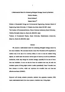
Figure 1. (a) Mie theory results of the backscattering ratio ˜ b bp as a function of the hyperbolic slope of the differential particle size distribution. (b) Results using a two-component particle size distribution comprised of gamma functions [Risovic, 1993]. Each curve in Figures 1a and 1b represent a different bulk refractive index, ranging between 1.02 and 1.20 at increments of 0.02. The imaginary part of the refractive index was held constant at 0.005. For the gamma-type distribution, comparable hyperbolic slopes of 3.5 and 4, calculated in the 1–20 m particle range, are represented by dashed lines in Figure 1b.
was the maximum radius when was small (relatively more large particles) and the refractive index was low. The limits used here were chosen so that scattering by particles with ␣ values outside these limits is expected to be negligible for any wavelength in the visible domain. After scattering properties were computed with Mie theory for each size they were
weighted according to a specific PSD and summed to obtain bulk estimates. Mie results with the two size distribution models were generally similar (Figures 1a and 1b). For values of ⱕ 3.6 and C S :C L ⬍ 10 14 , ˜ b bp was almost exclusively a function of refractive index. This implies that ˜ b bp and similar parameters
TWARDOWSKI ET AL.: LIGHT SCATTERING BY OCEAN PARTICLES
14,133
Figure 2. Mie theory results of ˜ b bp as a function of the imaginary part of the refractive index n⬘p . Each curve represents a different hyperbolic slope for the PSD, ranging from 2.5 (0.25) 4.5. The real part of the bulk refractive index was held constant at 1.04.
such as  (45⬚)/N 0 [Pak et al., 1970; Brown and Gordon, 1973a] may be used for obtaining n p with reasonably good accuracy under these conditions. For larger values of and C S :C L the models diverged. For the gamma size distributions, n p was important, and for the hyperbolic distributions both n p and the size distribution were important. At no reasonable value of or C S :C L was n p found to be unimportant. Thus the conclusion of Ulloa et al. [1994] that particle size distribution is the dominant factor controlling ˜ b bp only holds true for narrow ranges of n p . The two plateaus in the gamma distribution model at high C S :C L and low C S :C L represent regions where ˜ b bp is dominated by the small particle and large particle populations, respectively. The primary inconsistency in the two PSD models was for small particles (⬍1 m). Unfortunately, since measurements of particle sizes in the submicron range are very rare, there is limited knowledge of distributions ⬍1 m. Considering the scattering results computed with the two distribution models were generally similar, we found no justification for not using the typical hyperbolic model for the method. Caution must be exercised, however, in applying the model when estimated values (see section 3) are ⬎⬃4.2. The Mie theory results plotted in Figure 1a provided the foundation for our model for estimating n p . These relationships for the backscattering ratio were found to be spectrally independent in the visible, corroborating the theoretical findings of Ulloa et al. [1994] and the experimental observations by Macdonald et al. [2000]. The dependency of ˜ b bp on particle absorption was tested in the n⬘p range of 0.001– 0.1 (Figure 2). As n⬘p and values increased, ˜ b bp exhibited an increased dependency on n⬘p . In general, however, this dependency was minor for n⬘p values ⬍⬃0.01. A typical algal cell (a relatively strong absorber) is expected to have an n⬘p of ⬃0.0025– 0.005 [Morel and Bricaud,
1986; Kitchen and Zaneveld, 1992]. Typical n⬘p values for a bulk oceanic particle population are expected to be ⬍0.002 [Bricaud et al., 1995]. For these values of n⬘p the dependency of ˜ b bp on n⬘p generally varied ⬍5%. The effect of n⬘p was thus disregarded in the model. The reader is cautioned, however, that application of the model in a situation with a high average absorption per particle (weighted by absorption cross sections) will introduce an error.
3. Relationship Between Spectral Attenuation and Size Distribution Particulate attenuation spectra c p ( ) are characteristically smooth functions for polydisperse solutions of particles despite the fact that absorption spectra normally have strong and irregular (e.g., peaked) spectral dependencies in aquatic systems. This is because shape structure in an absorption spectrum is compensated by the inverse of such structure in the scattering spectrum. This is predicted by the theory of anomalous dispersion [van de Hulst, 1981]. Resulting c p spectra (a p ⫹ b p ) in marine waters therefore decrease monotonically with increasing wavelength according to a hyperbolic model, c p共 兲 ⫽ A c ⫺␥,
(12)
where ␥ is the hyperbolic slope of the spectrum and A c is the corresponding amplitude. It has long been recognized [Volz, 1954] that the shape parameter of the c p spectrum, ␥, is closely related to the shape of the particle size distribution for a polydispersion, where
␥ ⬇ ⫺ 3.
(13)
This relationship was noted by Morel [1973b] from Mie computations and was verified in a theoretical proof by Diehl and
14,134
TWARDOWSKI ET AL.: LIGHT SCATTERING BY OCEAN PARTICLES
Figure 3. Mie theory results for the dependence of the hyperbolic slope of the attenuation spectrum, ␥, on the slope of the PSD, . The solid line represents the ␥ ⫽ ⫺ 3 relationship, obtained when the Mie size parameter ␣ is fixed. The dashed curves were calculated with fixed minimum and maximum particle sizes. The curves with squares, crosses, and circles represent m p ⫽ 1.02 ⫺ 0i, m p ⫽ 1.20 ⫺ 0i, and m p ⫽ 1.02 ⫺ 0.01i, respectively. Haardt [1980] using the van de Hulst [1981] approximation of Mie theory. Studies have also observed empirical relationships between ␥ or spectral attenuation ratios and [Kitchen et al., 1982; Boss et al., 2001], although the relationships were not always predicted by ␥ ⬇ ⫺ 3 [Kitchen et al., 1982]. Some deviation from the ␥ ⬇ ⫺ 3 relationship was also observed in Mie computations by Kishino [1980] for a particle population with a bulk refractive index of 1.2. Consequently, it was of interest whether a rigorous relationship between and ␥ could be verified with Mie theory that could then be used to improve estimates of n p from the backscattering ratio in the model. For 1.02 ⱕ n p ⱕ 1.20 and 0.001 ⱕ n⬘p ⱕ 0.1, Mie computations of ␥ (fit over 440 – 650 nm) for 2.5 ⱕ ⱕ 5 with fixed ␣min and ␣max [Morel, 1973a, 1973b; Diehl and Haardt, 1980] followed the ⫺ 3 relationship exactly, within experimental error (Figure 3). This is not the preferred method of calculating spectral dependencies, however, because the particle diameter is not held constant (e.g., a given PSD for calculating c p ( 1 ) will shift by 2/1 in the calculation of c p ( 2 ) because ␣ ⬀ 1/). When particle diameter is kept fixed in the computations (so that ␣min and ␣max vary), the ⫺ 3 relationship was followed only for ⱖ 3.5. For values ⬍3.5 a nonlinearity was observed, with the estimated attenuation slope approaching an asymptote at zero. Little change was observed when n p was increased from 1.04 to 1.20 in the calculations (Figure 3). When an absorption component (n⬘p ) was added, a second nonlinearity was observed, this time for ⱖ 4.0. Therefore the only region where the ⫺ 3 relationship was maintained, regardless of changes in the complex refractive index, was for values between 3.5 and 4.0 (␥ values in the range 0.5–1.0). Since the majority of fitted ␥ values (⬎98% in the Gulf of California data set) fall within this range, the ⫺ 3 relationship was therefore adopted in our model.
4.
Model
An analytical model was developed to describe the Mie theory results from Figure 1a. The model solves for n p when b bp ⱕ 0.03: 2.5 ⱕ ⱕ 4.5 and 0 ⱕ ˜
Figure 4. Map of the Gulf of California with the locations of the 36 stations sampled. Stations 7, 17, and 33 are labeled.
⫺3兲2 ˜bp, 兲 ⫽ 1 ⫹ ˜ b 0.5377⫹0.4867共 关1.4676 ⫹ 2.2950共 ⫺ 3兲 2 n ˆ p共b bp
⫹ 2.3113共 ⫺ 3兲 4兴.
(14)
˜bp , ) predicted the n p from Mie theory The modeled n ˆ p (b with an average and median error of ⫾0.0035. The largest residuals, about 0.011, between the Mie calculations and the predicted values were in the region where approached 4.5 and ˜ b bp approached zero. After substituting (13) into (14) the final model was obtained: ␥兲 ˜bp, ␥ 兲 ⫽ 1 ⫹ ˜ n ˆ p共b b 0.5377⫹0.4867共 关1.4676 ⫹ 2.2950共 ␥ 兲 2 bp 2
⫹ 2.3113共 ␥ 兲 4兴.
5. 5.1.
(15)
Model Performance in the Gulf of California Study Area
Vertical profiles of hydrographic and optical parameters were collected at 36 locations throughout the Gulf of California in April 1999 (Figure 4). The gulf is ⬃1000 km long and 150 km wide. Maximum depths in the northern gulf are generally ⬍300 m, with a mean depth of about 200 m. For the rest of the gulf, south of the midrift islands, bottom depths are ⬎2 km everywhere except within 5–20 km of the coast. From November to May, areas around the midrift islands and along the east coast are the regions of highest productivity in the Gulf of California [Santamaria-del-Angel et al., 1994]. During this time the northern gulf is typically being continually mixed throughout the water column. This results from a combination of strong northwest winds, convection driven by solar heating, and tidal stirring from tidal amplitudes as high as 9 m [Hernandez-Ayon et al., 1993].
TWARDOWSKI ET AL.: LIGHT SCATTERING BY OCEAN PARTICLES
14,135
Figure 5. Profiles of optical parameters and chlorophyll concentration at an example case I location, station 17. In situ fluorescence counts were converted to chlorophyll concentrations on the basis of laboratory measurements in a culture of Thalassiosira weissflogii. The absolute magnitude should be treated as a rough (⫾50%) approximation.
5.2.
Optical Instrumentation and Methods
In situ hydrographic and optical parameters were measured with a ship-deployed profiling package. Conductivity, temperature, and depth parameters were measured with a SeaBird Sealogger conductivity-temperature-depth profiler (CTD) at 8 Hz. Chlorophyll fluorescence (blue excitation) was measured with a WETStar (WET Labs, Philomath, Oregon). Absorption and attenuation of all the in-water constituents except water, [a p ( ) ⫹ a diss()] and [c p ( ) ⫹ a diss()], were measured with an ac-9 (WET Labs). The ac-9 has dual 25 cm flow cells in which spectral absorption and attenuation are measured at nine wavelengths in the visible and near IR. A second ac-9 was used to measure a diss() by fitting a 0.2 m pleated maxicapsule filter (Gelman) to the intake of the absorption channel. Details of the method for ac-9 calibration, field use, and the application of corrections for temperature, salinity, scattering error, and time lags are described by Twardowski et al. [1999]. The ac-9s were calibrated daily by passing optically clean water (Barnstead, four-cartridge Nanopure system) through the flow cells under pressure. The near-IR (715 nm) subtraction method was used to correct the scattering error in the absorption measurements [Zaneveld et al., 1994]. Backscattering measurements were made with a Hydroscat-6 (HOBI Labs, Watsonville, California) at six wavelengths in the visible. The Hydroscat measures volume scattering at a nominal angle of 140⬚, (140⬚), and b b is estimated assuming a constant proportionality between (140⬚) and b b [⫽ 2(1.08)(140⬚)] [Maffione and Dana, 1997]. The sigma correction algorithm to correct for attenuation of the source beam [Maffione and Dana, 1997] was applied using the a t and c t measured with the ac-9 (a w and c w added to in situ measurements). The parameter K bb used in the third-order polynomial correction was estimated from (a t ⫹ 0.75b t ) (R. Maffione, personal communication, 1999). A WET Labs Super Modular Ocean Data and Power System
(SMODAPS) was used to power the instruments, acquire data, time stamp the data, and transmit the data up a single cable to an archiving computer. Buoyancy on the profiling package was balanced with flotation to provide a free-fall descent rate of 20 –50 cm s⫺1. The maximum possible deployment depth for the package was about 200 m. Measured optical parameters were used to derive the various IOPs using (4)–(6). The absorption and scattering coefficients of pure water were obtained from Pope and Fry [1997] and Morel [1974], respectively. The uncertainty in the ac-9 measurements is ⬃0.005 m⫺1 for both channels [Twardowski et al., 1999], although derived IOPs can have greater uncertainties because of error propagation through the calculations. After the final data set was prepared all data were binned to 1 m. 5.3.
Inherent Optical Properties for Representative Cases
Stations were grouped into case I and II water types by classifying all stations that were ⬎20 km from shore and ⬎400 m deep as case I (11 stations out of 36) and treating the rest as case II (Figure 4). The case I designation was intended to eliminate any waters that may experience influences from terrestrial runoff or bottom sediment resuspension/transport (i.e., to include only those waters where in situ processes affected the optical properties). For the Gulf of California, regional river discharge did not require consideration in such a designation. Profiles of scattering parameters and chlorophyll measured at a typical case I station are presented in Figures 5a–5c. A subsurface chlorophyll maximum was present with associated maxima in b p and b bp . Although b p and b bp generally had similar finescale structure, ˜ b bp varied markedly through the water column (Figure 5b). A factor of 3 increase in ˜ b bp with depth was common for case I stations, with the lowest ˜ b bp values, close to 0.005 (0.5% of total particulate scattering), in
14,136
TWARDOWSKI ET AL.: LIGHT SCATTERING BY OCEAN PARTICLES
Figure 6. Profiles of optical parameters and chlorophyll concentration at an example case II location, station 7.
the chlorophyll peak near the surface. The close inverse relationship between ˜ b bp and chlorophyll in surface waters was repeatedly observed at the case I stations. The a p /b p ratio is plotted as a proxy for the relative amount of pigmented particles (Figure 5c). A high a p /b p is normally representative of pigment-containing autotrophic particles that absorb relatively strongly. A low a p /b p is typically representative of organic tripton that absorbs weakly. Peaks in a p /b p were consistent with chlorophyll maxima. Both b p and b bp were generally much higher at case II stations, as demonstrated at stations 7 (Figure 6) and 33 (Figure 7). The profiles of b p and b bp usually had similar finescale structure but nonetheless exhibited marked variations in ˜ b bp with depth, as was observed in case I waters. The IOPs were generally very variable at the different case II stations. Station 7 was a case of increasing chlorophyll and ˜ b bp with depth, contrary to the trend at case I stations. Station 33 was a case of higher chlorophyll in surface waters and an inverse trend in chlorophyll and ˜ b bp with depth. In the measurements at both case I– and case II–type stations, any wavelength dependence of ˜ b bp was generally ⬍10% [Macdonald et al., 2000], supporting the theoretical predictions discussed earlier.
5.4.
Derived Parameters
5.4.1. Modeled bulk refractive index from ˜ bbp and cp(). The parameter was obtained from in situ c p ( ) measurements as described in section 4. The wavelengths 440, 488, 555, and 650 nm were used in the spectral fit of c p because these data had the most stable calibrations through the study period. ˜bp , ␥ ) based on (15) Profiles of derived (⫽ 3 ⫹ ␥) and n ˆ p (b at the example case 1 station and the two example case II stations (7 and 33) are plotted in Figures 8a– 8c. In all regions, derived fell within the range 3.5– 4.0. Since this was the linear region of the relationship between and ␥ (Figure 3), a more complex nonlinear relationship was not required to predict from ␥. At stations where the bottom depth was in the range of the profiler, values clearly decreased toward the bottom (e.g., Figure 8c). Similar observations have been made by Spinrad [1982], Barth et al. [1997], and Boss et al. [2001]. The parameter ˜bp , ␥ ) also increased toward the bottom in case II waters. n ˆ p (b Within chlorophyll peaks in case I waters (Figure 8a), minima ˜bp , ␥ ) were observed, with an increase in deeper waters in n ˆ p (b where tripton particles (nonalgal) presumably dominate. Including all the data collected in the Gulf of California,
Figure 7. Profiles of optical parameters and chlorophyll concentration at an example case II location, station 33.
TWARDOWSKI ET AL.: LIGHT SCATTERING BY OCEAN PARTICLES
14,137
˜bp , ␥ ) and estimated hyperbolic slope for each of the Figure 8. The estimated bulk refractive index n ˆ p (b profiles presented in Figures 5–7.
˜bp , ␥ ) ranged between 1.04 and 1.18 (Figure 9). Four n ˆ p (b specific groups of data were considered to illustrate the observed variability in bulk particle composition: (1) the case I stations below 100 m (group Id), (2) the case I stations at the chlorophyll maximum (group Ic), (3) the case II stations south
of the sill (group IIa), and (4) the bottom water at the case II stations north of the sill (group IId). For the Id group, ˜bp, ␥) values fell within the 1.10 and 1.12 contours den ˆ p(b spite the fact that both ˜ bbp and varied. This suggested that the particle composition was relatively constant below 100 m
˜bp , ␥ ) for four specific regions of the water column from the Figure 9. Estimated bulk refractive indices n ˆ p (b Gulf of California: (1) the case I stations below 100 m (Id), (2) the case I stations at the chlorophyll maximum (Ic), (3) the case II stations south of the sill (IIa), and (4) the bottom water at the case II stations north of the sill (IId). All data were meter-averaged except the Id group, where data were averaged to 5 m.
14,138
TWARDOWSKI ET AL.: LIGHT SCATTERING BY OCEAN PARTICLES
Figure 10. The relationship between bulk refractive index n p and ˜ b bp for hyperbolic slopes ranging between 2.5 (0.25) 3.5 (data from Figure 1a replotted and fitted). For these ranges of , n p was a strong function of ˜ b bp (regression given in text, equation (14)). despite changes in the relative size distribution of those particles. Within the chlorophyll peak at case I stations (group Ic), ˜ b bp and values fell in a very restricted area, characterized by ˜bp , ␥ ) values from 1.04 to 1.05 (Figure 9). This is the n p n ˆ p (b value expected for particles dominated by organic material, with a water content of ⬃60 –70% (that of living cells) [Aas, ˜bp , ␥ ) values were the lowest measured in 1996]. These n ˆ p (b the gulf. In contrast, bottom waters in the northern gulf (group IId) ˜bp , ␥ ) values. Backscatterexhibited the highest ˜ b bp and n ˆ p (b ing exceeded 2% of particulate scattering in some cases, and refractive index estimates ranged from 1.14 to 1.18. These ˜bp , ␥ ) values are characteristic of inorganic minerals, n ˆ p (b consistent with resuspension from the strong tidal stirring that occurs in this region [Alvarez-Borrego, 1983]. In case II waters south of the sill (group IIa), relatively wide ˜bp , ␥ ) ranges of ˜ b bp and were observed. Corresponding n ˆ p (b values ranged from 1.05, characteristic of case I waters within the chlorophyll maximum, to 1.15, characteristic of the bottom waters in the northern gulf. As a result, particle composition in these waters was likely very variable and strongly dependent on local circulation patterns, tidal influences, productivity, and sediment composition. 5.4.2. Modeled bulk refractive index from ˜ bbp only. Investigators have previously suggested that n p may be estimated with parameters similar to the backscattering ratio, including (45⬚) divided by the total number of particles [Pak et al., 1970; Brown and Gordon, 1973a] and (45⬚) divided by the total particulate surface area [Carder et al., 1974], and (140⬚)/ (10⬚) [Morel, 1973b]. We tested the accuracy of estimating n p from the backscattering ratio alone and compared the results with the more complete model presented in section 5.4.1. For ⬍ 3.5, n p could be derived with minimal error (⬍5%) from ˜ b bp alone (Figure 10): ˜bp兲 ⫽ 1 ⫹ 1.671b ˜0.582 n ˆ p共b bp ,
(16)
˜bp ) still predicted For values not much higher than 3.5, n ˆ p (b n p with a relatively small error. For example, in the estimated
Figure 11. Measured ˜ b bp as a function of measured chlorophyll. All data are plotted with crosses, with the case I data plotted with circle overlays. Curves representing the models of Gordon et al. [1988], Morel [1988], and Ulloa et al. [1994] are identified with a G, M, and U, respectively. The thick solid curve labeled GOC is the least-squares hyperbolic fit to the case I data. Intervals of 95% confidence are plotted as dashed curves around it. In the least-squares fitting procedure, 2 was minimized to 5.46 ⫻ 10⫺6, with a resulting correlation coefficient r 2 ⫽ 0.52. ranges of derived from c p ( ) in this study (3.5– 4.0), esti˜bp ) were never more than 20% different mates of n p using n ˆ p (b (after subtracting 1 from both) than estimates that used both ˜ b bp and ␥ in (15). At values of ⬎ 4, however, ˜ b bp rapidly increased for a given n p (Figure 1a), suggesting that estimates of n p with just ˜ b bp would rapidly become unacceptable.
6.
Relationship Between ˜ bbp and Chlorophyll
In bio-optical modeling for remote sensing of chlorophyll in case I waters, analytical approximations of spectral reflectance from the chlorophyllous pigment content of water require that relationships between b b and chlorophyll be estimated [e.g., Morel, 1988; Gordon et al., 1988]. Since the dependency of b on chlorophyll has been empirically determined in several studies (most recently by Loisel and Morel [1998]), b b is usually derived from b ˜ b bp , where ˜ b bp is modeled semianalytically as a function of chlorophyll [Morel, 1988; Gordon et al., 1988; Ulloa et al., 1994] or assumed to be constant [Sathyendranath and Platt, 1988]. We tested the dependency of ˜ b bp on chlorophyll with our direct in situ measurements (Figure 11). In general, our data fall in line with previous relationships from semianalytical models proposed by Gordon et al. [1988], Morel [1988], and Ulloa et al. [1994] (Figure 11). For the case I stations, ˜ b bp was a function of chlorophyll concentration, described with a hyperbolic model: ˜ b bp ⫽ 0.0096关chlorophyll兴 ⫺0.253,
(17)
with chlorophyll units of mg m⫺3. Although there was a statistically significant relationship between ˜ b bp and chlorophyll for the case I data, there was a large amount of scatter, particularly at low chlorophyll concentrations. This is consistent with the hypothesis that ˜ b bp is strongly a function of particle composition and that chlorophyllcontaining particles are not the only particles of importance.
TWARDOWSKI ET AL.: LIGHT SCATTERING BY OCEAN PARTICLES
At high chlorophyll levels, algal, low ˜ b bp (low n p ) particles dominate the scattering properties and the relationship between ˜ b bp and chlorophyll becomes tighter. At low chlorophyll levels in case 1 waters, ˜ b bp will be more dependent on the presence of nonpigmented particles (i.e., inorganic and organic tripton). Most of the values falling significantly above the modeled ˜ b bp ⫺ chlorophyll relationship were from case II–type waters and presumably contain a high proportion of inorganic particles. Most of the values falling significantly below the regression at low chlorophyll concentrations were from Case I–type waters. Particles in these waters were predominantly nonpigmented but with a bulk particle composition (n p ) similar to that of phytoplankton.
7. 7.1.
Discussion Analysis of Assumptions and Errors
For Mie theory to be applicable several assumptions were made about the particle population. The important assumptions were (1) a randomly oriented population of irregularly shaped particles can be approximated well by the equivalent size distribution of spherical particles and (2) heterogeneity in the internal structure of particles can be approximated by an “average” composition. These effects can change estimates of b b p by up to 30% under certain conditions [Kitchen and Zaneveld, 1992; Herring and Boss, 2000]. However, we are relatively optimistic that such errors are not large enough to discount the interpretation of the model results. A means of testing such errors is by observing how the model behaves through the chlorophyll maxima at the case I stations. Here the particle population will have a dominant component from living cells, which are characteristically nonspherical and mixed in internal composition [Thomas, 1997]. Theoretical predictions [Herring and Boss, 2000; Mishchenko et al., 1999] and laboratory measurements [Holland and Gagne, 1970; Shifrin, 1988] suggest that particles of irregular shape typically will have an increased backscattering ratio relative to equivalent spherical particles. Similarly, theory predicts that particles with layered interiors will have increased backscattering relative to particles with homogeneous interiors [Mueller, 1973; Bohren and Huffman, 1983; Kitchen and Zaneveld, 1992]. However, through the chlorophyll maxima the very lowest backscattering ratios were observed (about 0.005). Corresponding bulk refractive indices ranged from 1.04 to 1.05. Similar refractive indices have been estimated for phytoplankton on the basis of the macromolecular composition of algal cells [Aas, 1996], from culture analyses [Carder et al., 1972], and from VSF measurements made in productive marine waters [Roach, 1974; Zan˜bp , ␥ ) values are already eveld et al., 1974]. Since these n ˆ p (b low, backscattering, and, consequently, refractive index, could not have been substantially overestimated in this region. Overestimations of 0.01, or even 0.02, are not impossible, however. Another assumption that was made was a constant relationship between (140⬚), which was actually measured, and b b [Maffione and Dana, 1997]. Although making this assumption was not a necessity in this model, it gives the model universality, so when b b is derived by other methods, the model can still be used. To verify the results would have been the same if only (140⬚) was used,  (140⬚)/b p was computed from Mie theory as a function of the hyperbolic PSD slope and bulk refractive index instead of b bp /b p (as in Figure 1a). Estimates of n p were the same within about 5% after subtracting 1.
14,139
It must also be stated that the uncertainty in the estimate of (140⬚) (and thus b b ) with the Hydroscat is not well defined. In general, making accurate absolute measurements of the volume-scattering function is difficult. It is not unreasonable to suspect that these measurements could have an uncertainty of 5–10% [Pegau et al., 2001], which could translate into errors as high as 0.015 in estimating n p with the data considered here. Part of the utility of the backscattering ratio in the model, however, is that it spans a wide range under natural oceanic conditions, from about 0.002 to 0.030. Since estimated n p values range from 1.04 to about 1.18, a potential uncertainty of even 0.015 will not significantly change the interpretation of model results. 7.2. Model Results and Bulk Particle Composition in the Gulf of California The estimates of n p for groups Ic and IId agreed with expected values for algal cells and inorganic minerals, respectively. For the case II stations north of the midrift islands (e.g., ˜bp , ␥ ) values increased steadily with depth, Figure 8c), n ˆ p (b indicating an increased proportion of mineral particles relative to organic particles with depth. This is consistent with the fact that a source of inorganic minerals in the water column is bottom sediment resuspension and a source of particulate organic material is photosynthetic processes at the surface. For the case I stations below 100 m (group Id), where the optical properties of the particle population are most likely dominated by nonalgal tripton, we estimated an n p of 1.10 – 1.12. The increased refractive index relative to phytoplankton suggests two possible scenarios. First, the particles are composed primarily of organic tripton (dead organic material and living heterotrophs) with a lower water content (⬍40%) than phytoplankton. Alternatively, inorganic particles of high refractive index may significantly affect the scattering properties in these waters. The n p of organic tripton is not known, but it is reasonable to expect that certain types of organic tripton particles such as the fecal pellets of heterotrophic nanoplankton might have a relatively high n p because of their low water content. We are not aware of any directly measured values for organic tripton n p in the literature, but it can be roughly estimated using measurements of the volume and carbon content of detritus made by Verity et al. [1996]. In 15 samples, detrital organic carbon was estimated from detrital volume as 0.23 pg C m⫺3. If it is assumed that the detrital material that was analyzed was composed primarily of organic material, then the relationship between refractive index and particle carbon composition derived by Morel and Ahn [1990] for living cells (n p ⫽ 1 ⫹ 0.233 ⫻ 10 ⫺3 [C ip ], where [C ip ] is the organic carbon concentration in the particle in kg m⫺3) can be used to estimate the refractive index of organic tripton. The predominant factor influencing the conversion is the relation of water content in the particle to C ip . The resulting estimate of n p for the Verity et al. [1996] samples was 1.054, reflective of a relatively high water content (⬎60%), similar to that of phytoplankton. This is consistent with estimates of the refractive index of organic detrital particles made by Bricaud et al. [1995] off the Oregon coast. Bits of inorganic material such as coccoliths in the detrital particles would be expected to increase the estimate from the Verity et al. [1996] data. Although this analysis does not support the hypothesis that nonalgal organic particles significantly contribute to the relatively high n p of tripton, observations to this effect are currently very limited.
14,140
TWARDOWSKI ET AL.: LIGHT SCATTERING BY OCEAN PARTICLES
The hypothesis that inorganic minerals, both nonbiogenic and biogenic, may play an important role in scattering by tripton in many “case I” waters can be discussed in more detail. Using component analyses of VSFs collected in the 1960s by Gunnar Kullenburg in the Sargasso Sea, throughout the Mediterranean Sea, and in the central Baltic, Roach [1974] determined that scattering by a component with a refractive index of 1.15 was always significant, particularly at angles ⬎45⬚. Using similar component analyses, Brown and Gordon [1973b, 1974] came to the same conclusion. While minerals produced by algae and other organisms (e.g., calcite and amorphous silica) are readily observed in case I waters, direct experimental observations suggest that nonbiogenic inorganic minerals may be prevalent as well. The presence of nonbiogenic minerals has been observed at all depths in the west-central Gulf of Mexico [Harris, 1977] and Caribbean Sea [Jacobs and Ewing, 1965], off the southern California shelf [Wells and Goldberg, 1992], and in the eastern equatorial Pacific Ocean [Baker and Feely, 1978]. A significant source of this mineral fraction is aeolian inputs. Windom [1969] estimated that up to 75% of inorganic tripton in the Atlantic and Pacific Oceans is derived from atmospheric dust fallout based on similarities in composition between the minerals in the water column and that found in atmospheric dust and deep-sea sediments in the area. Atmospheric deposition of mineral particles has been shown to be substantial under certain conditions in the North Atlantic [Carder et al., 1986]. The Gulf of California, specifically, is surrounded by an arid landscape, which can be expected to be a source of terrigenous dust to surface waters. Aeolian inputs may be significant in the winter season when the winds are from the northwest, over the Baja mountain range. It is thus a distinct possibility that nonbiogenic minerals are a significant source of scattering (particularly backscattering) for waters in the Gulf of California that were designated case I in this study. The global effect of such inputs on scattering properties remains to be determined. A hypothesis consistent with our observations is that there are three primary components important for backscattering in waters that were designated case I: algal cells (n p of 1.04 – 1.05), organic tripton (n p of roughly 1.05), and inorganic tripton (n p of 1.14 –1.18). These components are clearly represented in the ˜ b bp -chlorophyll plot in case I waters (Figure 11). At low chlorophyll concentrations, ˜ b bp varied over a wide range, 0.004 – 0.022, in agreement with an analysis by Sathyendranath et al. [1989] of spectral reflectance measurements in case I waters. When ˜ b bp was low for these chlorophyll levels, organic tripton (dead cell material and/or living heterotrophs) was likely dominating ˜ b bp . When ˜ b bp was high, it is likely that inorganic tripton (biogenic and/or nonbiogenic minerals) was important. As a final note, the possible presence of a significant nonbiogenic mineral fraction is inconsistent with the formal definition of case I waters, which presupposes a negligible concentration of these particles, i.e., that the only optically significant materials besides water itself are phytoplankton and phytoplankton-derived materials. One might thus be inclined to classify all of the Gulf of California as case II if aerosol-derived inorganic minerals are indeed an important source of backscattering. It must be considered, however, that other analyses of VSF measurements made in waters normally considered case I (e.g., Sargasso Sea and central Mediterranean) have concluded that inclusion of a mineral-like component in the
particle population was necessary to describe observed levels of backscattering [Brown and Gordon, 1973b, 1974; Roach, 1974; Zaneveld et al., 1974]. Also important in this regard is that the ˜ b bp in ˜ b bp -chlorophyll relationships used in semianalytical remote sensing models for case I waters (see Figure 11) is typically not constant at a reasonable value for phytoplankton (around 0.5%). It is unclear at this point if the increase in ˜ b bp with decreasing chlorophyll may be incorporating an influence from nonbiogenic inorganic minerals in some case I algorithms or if organic detrital particles with low water content are, in fact, often important. Investigations into the scattering properties and composition of naturally occurring tripton from many regions are needed to make this determination.
Notation a x absorption coefficient, where x ⫽ t, w, p, and diss specifies total, water, particulate, and dissolved, respectively, m⫺1. A n amplitude of hyperbolic fit to N( ␣ ), m⫺3. A c amplitude of hyperbolic fit to c p spectrum, m⫺1. ␣ Mie size parameter, dimensionless. ␣ min, ␣max upper and lower limits of integration for the particle size distribution; are a function of wavelength, dimensionless. b x scattering coefficient, where x ⫽ t, w, p, b, f, and bp specifies total, water, particulate, backward, forward, and backward particulate, respectively, m⫺1. ˜ b bp particulate backscattering ratio, dimensionless.  volume scattering coefficient, sr⫺1 m⫺1. c x attenuation coefficient, where x ⫽ t, w, and p specifies total, water, and particulate, respectively, m⫺1. C ip organic carbon concentration for a particle kg m⫺3. C S , C L proportionality constants of the relative concentrations of a small and a large particle population described by a gamma distribution. E irradiance, W m⫺2. F( ␣ ) particle size distribution function, m⫺4. ␥ hyperbolic slope of c p spectrum, dimensionless. i⬜(, m, ␣), i储(, m, ␣) parallel and perpendicular components of scattering intensity, dimensionless. I radiant intensity, W sr⫺1. K bb sigma correction parameter, m⫺1. wavelength, m or nm. m p complex particulate refractive index, dimensionless. S, L, bS, bL, ␥S, ␥L parameters describing the modal value, width, and skewness of the small and large gamma distributions, dimensionless, except for b S and bL parameters, m⫺1. n p real part of the particulate refractive index, dimensionless. n⬘p imaginary part of the particulate refractive index, dimensionless. n p bulk particulate refractive index (real part), dimensionless.
TWARDOWSKI ET AL.: LIGHT SCATTERING BY OCEAN PARTICLES
˜bp , ␥ ) modeled bulk particulate refractive index as a n ˆ p (b function of the backscattering ratio and slope of spectral attenuation, dimensionless. ˜bp ) modeled bulk particulate refractive index as a n ˆ p (b function of the backscattering ratio, dimensionless. N( ␣ ) particle size distribution, m⫺3. N 0 total concentration of particles, m⫺3. Q x optical efficiencies, where x ⫽ b, b b , and c specifies scattering, backscattering, and attenuation, respectively, dimensionless. angle, radians. r radius, m. r m modal radius of gamma distribution, m. V volume, m⫺3. hyperbolic slope of particle size distribution, dimensionless. Acknowledgments. The authors thank Kusiel Shifrin, Robert Stavn, and two anonymous reviewers for valuable comments on the manuscript. Helmut Maske and the crew of the B/O Francisco de Ulloa are graciously acknowledged for assistance in data collection. M.S.T. received partial support from an Environmental Optics Postdoctoral Fellowship from WET Labs, Inc. Additional financial support was provided by the NASA SIMBIOS program and the ONR Environmental Optics program.
References Aas, E., The refractive index of phytoplankton, Rep. 46, 61 pp., Inst. Geophys., Univ. of Oslo, Oslo, Norway, 1981. Aas, E., Refractive index of phytoplankton derived from its metabolite composition, J. Plankton Res., 18, 2223–2249, 1996. Ackleson, S. G., and R. W. Spinrad, Size and refractive index of individual marine particulates: A flow cytometric approach, Appl. Opt., 27, 1270 –1277, 1983. Alvarez-Borrego, S., Gulf of California, in Estuaries and Enclosed Seas, edited by B. H. Ketchum, pp. 427– 449, Elsevier Sci., New York, 1983. Bader, H., The hyperbolic distribution of particle sizes, J. Geophys. Res., 75, 2822–2830, 1970. Baker, E. T., and R. A. Feely, Chemistry of oceanic particulate matter and sediments: Implications for bottom sediment resuspension, Science, 200, 533–534, 1978. Barth, H., K. Grisard, K. Holtsch, R. Reuter, and U. Stute, Polychromatic transmissometer for in-situ measurements of suspended particles and gelbstoff in water, Appl. Opt., 36, 7919 –7928, 1997. Bohren, C. J., and D. R. Huffman, Absorption and Scattering of Light by Small Particles, 530 pp., John Wiley, New York, 1983. Boss, E., W. S. Pegau, W. D. Gardner, J. R. V. Zaneveld, A. H. Barnard, M. S. Twardowski, G. C. Chang, and T. D. Dickey, The spectral particulate attenuation and particle size distribution in the bottom boundary layer of a continental shelf, J. Geophys. Res., 106, 9509 –9516, 2001. Bricaud, A., C. Roesler, and J. R. V. Zaneveld, In situ methods for measuring the inherent optical properties of ocean waters, Limnol. Oceanogr., 40, 393– 410, 1995. Brown, O. B., and H. R. Gordon, Comment on “Method for the determination of the index of refraction of particles suspended in the ocean,” J. Opt. Soc. Am., 63, 1616 –1617, 1973a. Brown, O. B., and H. R. Gordon, Two component Mie scattering models of Sargasso Sea particles, Appl. Opt., 12, 2461–2465, 1973b. Brown, O. B., and H. R. Gordon, Size-refractive index distribution of clear coastal water particulates from light scattering, Appl. Opt., 13, 2874 –2881, 1974. Carder, K. L., Particles in the eastern equatorial Pacific Ocean: Their distribution and effect upon optical parameters, Ph.D. thesis, Oregon State Univ., Corvallis, 1970. Carder, K. L., R. D. Tomlinson, and G. F. Beardsley Jr., A technique for the estimation of indices of refraction of marine phytoplankters, Limnol. Oceanogr., 17, 833– 839, 1972.
14,141
Carder, K. L., P. R. Betzer, and D. W. Eggimann, Physical, chemical, and optical measures of suspended particle concentrations: Their intercomparison and application to the west African shelf, in Suspended Solids in Water, edited by R. J. Gibbs, pp. 173–193, Plenum, New York, 1974. Carder, K. L., R. G. Steward, and P. R. Betzer, Dynamics and composition of particles from an aeolian input event to the Sargasso Sea, J. Geophys. Res., 91, 1055–1066, 1986. Diehl, P., and H. Haardt, Measurement of the spectral attenuation to support biological research in a “plankton tube” experiment, Oceanol. Acta, 3, 89 –96, 1980. Gordon, H. R., O. B. Brown, R. H. Evans, J. W. Brown, R. C. Smith, K. S. Baker, and D. K. Clark, A semianalytical radiance model of ocean color, J. Geophys. Res., 93, 10,909 –10,924, 1988. Grams, G. W., I. H. Blifford Jr., D. A. Gillette, and P. B. Russell, Complex index of refraction of airborne soil particles, J. Appl. Meteorol., 13, 459 – 471, 1974. Harris, J. E., Characterization of suspended matter in the Gulf of Mexico, II, Particle size analysis of suspended matter from deep water, Deep Sea Res., 24, 1055–1061, 1977. Hernandez-Ayon, J. M., M. S. Galindo-Bect, B. P. Flores-Baez, and S. Alvarez-Borrego, Nutrient concentrations are high in the turbid waters of the Colorado River Delta, Estuarine Coastal Shelf Sci., 37, 551–561, 1993. Herring, S., and E. Boss, Optical properties of non-spherical marine particles, Eos Trans. AGU, 80(49), Ocean Sci. Meet. Suppl., OS22806, 2000. Holland, A. C., and G. Gagne, The scattering of polarized light by polydisperse systems of irregular particles, Appl. Opt., 9, 1113–1121, 1970. Hunt, J. R., Prediction of oceanic particle size distributions from coagulation and sedimentation mechanisms, in Advances in Chemistry Series, vol. 189, Particulates in Water, edited by M. C. Kavanaugh and J. O. Leckie, pp. 243–257, Am. Chem. Soc., Washington, D. C., 1980. Jacobs, M. B., and M. Ewing, Mineralogy of particulate matter suspended in sea water, Science, 149, 179 –180, 1965. Jonasz, M., Particle size distributions in the Baltic, Tellus, Ser. B, 35, 346 –358, 1983. Kishino, M., Studies of the optical properties of sea water: Application of Mie theory to suspended particles in sea water, Sci. Pap. Inst. Phys. Chem. Res. Jpn., 74, 31– 45, 1980. Kitchen, J. C., Particle size distributions and the vertical distribution of suspended matter in the upwelling region off Oregon, Rep. 77-10, 118 pp., Oregon State Univ., Corvallis, 1977. Kitchen, J. C., and J. R. V. Zaneveld, A three-layered sphere model of the optical properties of phytoplankton, Limnol. Oceanogr., 37, 1680 –1690, 1992. Kitchen, J. C., J. R. V. Zaneveld, and H. Pak, Effect of particle size distribution and chlorophyll content on beam attenuation spectra, Appl. Opt., 21, 3913–3918, 1982. Lide, D. R. (Ed.), Physical and optical properties of minerals, in CRC Handbook of Chemistry and Physics, 77th ed., pp. 4.130 – 4.136, CRC Press, Boca Raton, Fla., 1997. Loisel, H., and A. Morel, Light scattering and chlorophyll concentration in case 1 waters: A reexamination, Limnol. Oceanogr., 43, 847– 858, 1998. Macdonald, J. B., M. S. Twardowski, W. S. Pegau, A. H. Barnard, E. Boss, and J. R. V. Zaneveld, Characterization of spectral backscattering in the Gulf of California, Eos Trans. AGU, 80(49), Ocean Sci. Meet. Suppl., OS22E-12, 2000. Maffione, R. A., and D. R. Dana, Instruments and methods for measuring the backward-scattering coefficient of ocean waters, Appl. Opt., 36, 6057– 6067, 1997. Mishchenko, M. I., J. W. Hovenier, and L. D. Travis (Eds.), Light Scattering by Nonspherical Particles, 690 pp., Academic, San Diego, 1999. Morel, A., Indicatrices de Diffusion Calculees par la Theorie de Mie pur les Systems Polydisperses, en vue de l’Application aux Particules Marines, Rep. 10, 75 pp., Lab. d’Oceanogr. Phys., Univ. de Paris VI, Paris, 1973a. Morel, A., Diffusion de la lumiere par les eaux de mer: Resultats experimentaux et approche theorique, in Optics of the Sea, AGARD Lecture Ser., vol. 61, pp. 3.1.1–3.1.76, North Atlantic Treaty Org., Brussels, 1973b. Morel, A., Optical properties of pure water and pure seawater, in
14,142
TWARDOWSKI ET AL.: LIGHT SCATTERING BY OCEAN PARTICLES
Optical Aspects of Oceanography, edited by N. G. Jerlov and E. Steemann Nielson, pp. 1–24, Academic, San Diego, Calif., 1974. Morel, A., Optical modeling of the upper ocean in relation to its biogenous matter content (case I waters), J. Geophys. Res., 93, 10,749 –10,768, 1988. Morel, A., and Y.-H. Ahn, Optical efficiency factors of free-living bacteria: Influence of bacterioplankton upon the optical properties and particulate carbon in oceanic waters, J. Mar. Res., 48, 145–175, 1990. Morel, A., and A. Bricaud, Inherent properties of algal cells including picoplankton: Theoretical and experimental results, Can. Bull. Fish. Aquatic Sci., 214, 521–559, 1986. (Reproduced in Photosynthetic Picoplankton, edited by T. Platt and W. K. W. Li, Dept. of Fish. and Oceans, Ottawa, Ont., Can., 1986.) Mueller, J. L., The influence of phytoplankton on ocean color spectra, Ph.D. thesis, 239 pp., Oregon State Univ., Corvallis, 1973. Pak, H., G. F. Beardsley Jr., G. R. Heath, and H. Curl, Light scattering vectors of some marine particles, Limnol. Oceanogr., 15, 683– 687, 1970. Patterson, E. M., D. A. Gillette, and B. H. Stockton, Complex index of refraction between 300 and 700 nm for Saharan aerosols, J. Geophys. Res., 82, 3153–3160, 1977. Pegau, W. S., E. Boss, A. Weidemann, G. Korotaev, M. Lee, and E. Shibanoy, Measurements of the backscattering coefficient, paper presented at American Society for Limnology and Oceanography Meeting, Albuquerque, N. M., February 12–16, 2001. Pope, R. M., and E. S. Fry, Absorption spectrum (380 –700 nm) of pure water, II, Integrating cavity measurements, Appl. Opt., 36, 8710 – 8723, 1997. Risovic, D., Two-component model of sea particle size distribution, Deep Sea Res., Part I, 40, 1459 –1473, 1993. Roach, D. M., Determination of refractive index distributions for oceanic particulates, Ph.D. thesis, 172 pp., Oregon State Univ., Corvallis, 1974. Santamaria-del-Angel, E., S. Alvarez-Borrego, and F. E. MullerKarger, Gulf of California biogeographic regions based on coastal zone color scanner imagery, J. Geophys. Res., 99, 7411–7421, 1994. Sathyendranath, S., and T. Platt, The spectral irradiance field at the surfaces of the ocean: A model for application and in the interior in oceanography and remote sensing, J. Geophys. Res., 93, 9270 –9280, 1988. Sathyendranath, S., L. Prieur, and A. Morel, A three-component model of ocean colour and its application to remote sensing of phytoplankton pigments in coastal waters, Int. J. Remote Sens., 10, 1373–1394, 1989. Shifrin, K., Physical Optics of Ocean Water, 285 pp., Am. Inst. of Phys., New York, 1988. Spinrad, R. W., Optical characteristics of the suspended sediment in the high energy benthic boundary layer experiment, Ph.D. thesis, 134 pp., Oregon State Univ., Corvallis, 1982.
Spinrad, R. W., and J. F. Brown, Relative real refractive index of marine microorganisms: A technique for flow cytometric estimation, Appl. Opt., 25, 1930 –1934, 1986. Stramski, D., and D. A. Kiefer, Light scattering by microorganisms in the open ocean, Prog. Oceanogr., 28, 343–383, 1991. Stramski, D., A. Morel, and A. Bricaud, Modeling the light attenuation and scattering by spherical phytoplankton cells: A retrieval of the bulk refractive index, Appl. Opt., 27, 3954 –3956, 1988. Thomas, C. R. (Ed.), Identifying Marine Phytoplankton, 858 pp., Academic, San Diego, Calif., 1997. Twardowski, M. S., J. M. Sullivan, P. L. Donaghay, and J. R. V. Zaneveld, Microscale quantification of the absorption by dissolved and particulate material in coastal waters with an ac-9, J. Atmos. Oceanic Technol., 16, 691–707, 1999. Ulloa, O., S. Sathyendranath, and T. Platt, Effect of the particle-size distribution on the backscattering ratio in seawater, Appl. Opt., 33, 7070 –7077, 1994. van de Hulst, H. C., Light Scattering by Small Particles, 470 pp., Dover, Mineola, N. Y., 1981. Verity, P. G., T. M. Beatty, and S. C. Williams, Visualization and quantification of plankton and detritus using digital confocal microscopy, Aquat. Microb. Ecol., 10, 55– 67, 1996. Volz, F., Die Optik und Meterologie der atmospharischen Trubung, in Ber. des Detsch. Wetterdienstes 13, vol. 2, pp. 3– 47, Bad Kissingen, Germany, 1954. Wells, M. L., and E. D. Goldberg, Marine submicron particles, Mar. Chem., 40, 5–18, 1992. Windom, H. L., Atmospheric dust records in permanent snowfields: Implications to marine sedimentation, Geol. Soc. Am. Bull., 80, 761–782, 1969. Zaneveld, J. R. V., and H. Pak, Method for the determination of the index of refraction of particles suspended in the ocean, J. Opt. Soc. Am., 63, 321–324, 1973. Zaneveld, J. R. V., D. R. Roach, and H. Pak, The determination of the index of refraction distribution of oceanic particulates, J. Geophys. Res., 79, 4091– 4095, 1974. Zaneveld, J. R. V., J. C. Kitchen, and C. M. Moore, The scattering error correction of reflecting-tube absorption meters, in Ocean Optics XII, Proc. SPIE Int. Soc. Opt. Eng., 2258, 44 –55, 1994. A. H. Barnard, E. Boss, J. B. Macdonald, W. S. Pegau, and J. R. V. Zaneveld, College of Oceanic and Atmospheric Sciences, Oregon State University, Corvallis, OR 97331. M. S. Twardowski, Department of Research, WET Labs, Inc., P.O. Box 468, Saunderstown, RI 02874-0468. (
[email protected])
(Received April 6, 2000; revised January 29, 2001; accepted February 13, 2001.)