overcome channel outages and [6], [7] optimize resource utilization in vehicular ..... Interference plus Noise Ratio (SINR) γ, and N: T = gT (Î,N) ..... [23] P. A. Zandbergen, âAccuracy of iPhone locations: A comparison of assisted GPS, WiFi and ...
1
A Model for Throughput Prediction for Mobile Users Nicola Bui12 , Foivos Michelinakis12 , Joerg Widmer1 1 IMDEA Networks Institute, Madrid, Spain 2 Universidad Carlos III de Madrid (UC3M), Madrid, Spain
Abstract—In this paper we propose a stochastic model to predict user throughput in mobile networks. In particular, the model accounts for uncertainty such as random phenomena (e.g., fast fading) or inexact information (e.g., user location) to derive the statistical distribution of the user throughput. Such a model is highly useful for aiding scheduling and resource allocation decisions. In addition, we provide a taxonomy of prediction techniques to investigate error sources and the main characteristics of prediction accuracy. Finally, we show the versatility of the model by analyzing LTE user throughput for the case where knowledge of either the user’s actual position or the congestion level in the cell is inexact.
I.
I NTRODUCTION
The rapid growth of mobile traffic volume [1] is taxing the capacity of current mobile networks and poses a significant problem for mobile operators. Augmenting the network capacity to cope with this traffic or offloading the traffic to other wireless technologies such as WLAN may not always be the best solution since the former is very costly and the latter may not work in all cases [2], [3]. As a consequence, it is highly important to try to reduce traffic volume and increase network efficiency (while at the same time rolling out faster mobile networks). In this context, it is beneficial to leverage forecasted user throughput to improve the resource allocation and to reduce cell congestion. For instance, the Piecewise Constant Threshold (PCT) algorithm [4] sends more data when the signal quality (i.e., the Signal to Interference and Noise Ratio – SINR) is high, while primarily relying on buffered data while it is low. Similarly, [5] adopts an anticipatory scheduling algorithm to forecast and overcome channel outages and [6], [7] optimize resource utilization in vehicular environments. All of these solutions aim at scheduling traffic when capacity is abundant, so that congestion is reduced and, consequently, fewer resources are needed to serve the overall traffic volume. The above works depend on the capability of predicting the future resource availability and many of them in fact analyze their algorithm’s performance under the assumption of perfect knowledge. Network predictability is thoroughly studied, for example, in [8]. This work also affirms that cellular network data shows a high level of self-similarity and user “mobility directly impacts resource usage.” Thus, being able to model [9] and forecast [10] human mobility patterns aids predicting network resource availability for mobile users. The main contribution of this paper is a novel synthetic model representing the impact of estimation and prediction errors on the bandwidth availability statistics to be able to
study network resource optimization problems under forecasting uncertainties. In order for the model to account for the many different error sources, we analyze state of the art prediction models for both network resources as well as user mobility, which we subsequently organize in a taxonomy based on the time-scale and granularity of the prediction. The rest of the paper is structured as follows. Section II provides an overview and taxonomy of predictors upon which our model is based. In Section III, we discuss in detail the model for network resource availability under estimation and prediction errors. The model is applied to LTE cellular systems in Section IV. Finally, Section V concludes the paper. II.
TAXONOMY OF P REDICTORS
In this section, we analyze predictors for both user mobility (II-A) and network resource availability (II-B) in order to understand the forecasting capability for mobile systems and the accuracy of the available solutions. The considered works cover a wide range of time scales, location granularities and levels of accuracy. To provide a comprehensive model, we classify them in three categories according to their time and space granularity. The first group [11]–[14], (1)-net, is the most coarse: network performance is modeled by analyzing the whole network at once, with a time scale on the order of minutes to hours; users are statistically mapped to base station cell ID or geographic location, i.e., predictions obtained by these models concern average throughput achievable in the location a given user is most likely to be found. Algorithms in the second group [15]–[18], (2)-cell, combine user mobility information and network location specific information to refine prediction granularity. Predictors belonging to this group aim at predicting the next cell a user is likely to visit, the congestion level in that cell and the time of the visit. Its timescale is between tens of seconds and a few minutes. The third group [19]–[22], (3)-user, comprises the predictors with highest time granularity: in fact, most of the solutions in this group leverage filtering techniques and historical data. The aim, here, is to model the fast bandwidth variations experienced by the users on a timescale of tens of milliseconds up to a few seconds. Table I groups the papers into the three categories and also provides a high level description of the papers. The “Cat.” column specifies the name of the category, while the “Accuracy” column provides an evaluation of the effectiveness of the techniques. Here, we use the ratio between the mean square error of the prediction and the standard deviation of the original
2
TABLE I.
(2)-cell
(1)-net
Cat.
(3)-user
Ref. [11] [12] [13] [14] [15] [16] [17] [18] [19] [20] [21] [22]
Accuracy cr ∼ 0.8 ε ∼ 0.15 ε ≥ 0.01 ε ∈ [0.01 − 1] cr ∈ [0.5 − 0.72] εl ∼ 2 m cr ∈ [0.2 − 0.7] cr > 0.8 ε ∈ [0.05 − 2] ε∼1 n/a ε ∼ 0.01
P REDICTION TAXONOMY
Notes Provides a model for the number of user in a cell. ARIMA models and wavelet MRA. GARCH-ARIMA accurately models static high-speed network traffic. Evaluates multi scale and s-sample prediction. Compares Markovian (better) and Lempel-Ziv models. User trajectory prediction. Route prediction on GPS data. Using pre-filtered data and Markov models. Prediction possible in the 98% of the cases. Empirical study on user traces using wavelet approximations and filtering. First attempt at mobile system bandwidth prediction. Complete solution for mobile bandwidth forecast. Spatial and temporal dynamics characterization of mobile Internet traffic.
time series (e.g.: the user throughput, the bandwidth availabil∑ ∑ ity, etc.) ε = MSE(˜ x)/σx2 = i (xi − x ˜i )2 / i (xi − µx )2 , where xi and x ˜i are the i-th samples of the original time series and their predictions, respectively, and σx and µx are the standard deviation and the average of the original time series, respectively; cr is the correct prediction rate defined as the ratio between the number of times the predicted location of a user is correct and the number of attempts; and εl represents the distance between the predicted and the correct user position. A. Mobility Predictors The most common methods to locate a mobile terminal are, in order of decreasing accuracy, the Global Positioning System (GPS), WiFi, and cellular network positioning. These solutions can identify a terminal’s position with an average error on the order of 10, 100 and 500 meters, respectively [23]. Theoretical works, such as [9] and [10] studied characteristics of human behavior and found that an appreciable level of self-similarity exists among behavioral patterns and that, within due limits, forecasting is possible. Among the many studied properties, we highlight the one asserting that the probability of a user to be found in a given location is approximately inversely proportional to the location rank. Some predictors aim at estimating the next user position on a grid representing network cells: [15](2) compares Markovian and Lempel-Ziv models trained with the sequences of locations a user visited in the past, while [11](1) studies the accuracy of mobility modeling. Notably, the first paper comes to the conclusion that second order Markov models provide a good trade off between complexity and accuracy achieving a correct prediction rate cr ∈ [0.5 − 0.72] on mobility traces collected from more than 6000 users of Dartmouth College’s wireless network. The second paper provides an effective way to estimate the number of users in a cell and, consequently, the congestion level. Other predictors deal with routes and trajectories. [16](2) uses 1-sample predictions of user position to improve the performance of a routing protocol. (An s-sample prediction computes the first s unknown samples of a given time series.) The location prediction accuracy is claimed to be on the order of a few meters, with a position error εl ∼ 2 m. The work in [17](2) focuses on predicting complete routes from historical GPS data and obtains a cr ∈ [0.2 − 0.7]. Here, the best results are obtained when excluding single trips from the dataset.
Finally, [18](2) uses second and third order Markov models trained on a pre-filtered leap graph to model and predict cellular user mobility. The solution is able to achieve a cr ≥ 0.8 in 98% of the cases. Finally, recent works, such as [7] and [21](3) , directly exploit position information obtained from navigation systems to map bandwidth availability to locations. While these solutions provide a prediction that is based on the actual intended destination of the user, the accuracy of the prediction is still limited by the accuracy of the positioning system and the possibility of user detours. To the best of our knowledge, a detailed study linking location prediction accuracy to bandwidth/throughput prediction accuracy does not exist. B. Bandwidth Predictors One of the most relevant studies on traffic dynamics for cellular networks is [8], which conducted the first detailed wide scale analysis of network usage and subscriber behavior. The paper characterizes mobility and temporal activity patterns and identifies their relation to traffic volume. Traffic has been analyzed from the base station point of view, identifying its variations over space and time. Earlier works such as [12](1) , [19](3) and [13](1) studied different filtering techniques, namely MEAN, LAST, BM, MA, AR, ARMA, ARIMA, and FARIMA, all of which are different combinations of moving average and autoregressive filtering. We refer the interested reader to the source papers for the details. Although different papers use slightly different metrics, the following conclusions can be drawn: low order filtering techniques coupled with smoothing solutions (e.g., wavelet MultiResolution Analysis (MRA) or wavelet approximation) are able to provide 1-sample static network traffic predictions with an error as low as ε = 0.05 and almost always lower than the variance of the original signal, ε = 1. (In the latter case, the predicted sample error would be as large as those that would have been obtained by generating random samples from a distribution with the same variation as the original signal). The error decreases with larger timescale and smoother approximation of the signal. Subsequent work in [14](1) compares FARIMA and GARCH filtering techniques in terms of both time scale and the number of predicted samples s. Results obtained from Internet traffic traces show that GARCH outperforms FARIMA, achieving an error that is four time smaller. The
3
authors confirm that the error decreases with increased signal timescales and increases with the number of predicted samples s. In particular, the error becomes as high as the variance of the original signal for s = 10 and s = 100 samples for FARIMA and GARCH, respectively. Also, GARCH errors are slightly smaller than half the variance for s = 10 samples and beyond. [20](3) and [22](3) study resource availability in mobile systems. The former observes no significant correlation within a single trip, but throughput traces show a higher degree of self-similarity during repeated trips. The latter paper, instead, classifies traffic according to spatial features and proposes a multi-class model to predict traffic, achieving promising results (ε ∼ 0.01). Finally, although standard filtering techniques for static environments are less effective when applied to throughput of mobile nodes, they provide better accuracy when location is used as a context. III. BANDWIDTH AVAILABILITY M ODEL Based on the previous taxonomy, this section determines the main error sources and their impact on the statistical distribution of the predicted throughput. Fig. 1 shows examples of effects of errors on throughput prediction: the x-axis represents how far into the future the prediction is made, while the y-axis represents the predicted throughput and the corresponding estimation error. Note that purpose of the figure is to graphically exemplify the predictor categories; it is primarily intended to provide an intuition.
200
Bandwidth
T = gT (Γ, N ) = T0 η/N,
150
100
50 Cat.3
Cat.2 1s
Cat.1 1m
1h
Time
Fig. 1. Bandwidth forecasting examples: category 3, 2 and 1 predictor outputs are shown on the left hand side, in the center and on the right hand side, respectively.
The figure examines the three categories of the taxonomy starting from (3)-user category on the left hand side. Here, the solid line represents the prediction itself, while the two dashed lines represent the confidence range of the prediction. Although the accuracy degrades with time, predictors belonging to this category are able to closely follow the throughput variations. As soon as the confidence range becomes as large as the signal’s standard deviation, category (2)-cell predictors becomes as effective as category (3)-user predictors. In the center, predictions obtained from the category (2)cell are shown. Here, the predictions are averaged over longer
(1)
where Γ = 10 log10 γ is the SINR in dB, T0 is a parameter specific to the actual cellular system and η = gη (Γ) is the spectral efficiency for that SINR. The SINR is a function of d and the fast fading gain r: γ = gγ (d, r) = γ0 r/dα ,
250
0 0
time periods and their variability is represented by error bars. The solid line represents the actual prediction average along with its standard deviation, while the dashed line represents the same for the original signal. Predictors in this category infer user throughput from their position and statistics of the corresponding network cell. Whenever it is not possible to predict the next user location, only predictors in category (1)-net can be used (right hand side of Fig. 1). They derive an estimate of user throughput from general network information using, for example, the generic distribution of user throughput in the overall network (shown in the figure as a dashed line). To model the impact of errors on the predictors, we start from a simple formulation of the phenomenon itself. A very popular user throughput model can be found, for instance, in [24]. Here, the throughput T of a user with a distance of d kilometers to the transmitter and competing with N other users uniformly distributed within the coverage area of the transmitter, is represented as a function of the Signal to Interference plus Noise Ratio (SINR) γ, and N :
(2)
where γ0 is a technology specific parameter and α is the pathloss exponent. For what concerns errors themselves, different predictors are impacted by different error sources: for instance, those belonging to the third category try to model the short term behavior of the achievable throughput starting from past information. Thus, predicted throughput T˜ = T + eT , is the sum of the actual throughput and the prediction erro. Given that the error eT has a probability density function (pdf) feT (e), the predicted throughput will have a pdf fT˜ = feT (e − T ). Also, in the worst case the s-sample prediction can be modeled has the sum of s i.i.d random variables with distribution feT (e). Thus the s-sample predicted throughput distribution can be obtained as fT˜(s) = feT ((e − T )/s)/s, which will have an expected value µT˜(s) = T (s) + sµeT and standard deviation σT˜(s) = sσeT . Note that increasing s makes the prediction less and less accurate up to a point where the standard deviation of the prediction becomes comparable to the variability of the throughput σT . Beyond this point using this type of predictors is useless and category 2 and category 1 predictors should be used. In this case, most of the predictors try to first estimate system parameters, such as the distance d and the number N of users and, from those, estimate the throughput distribution. Thus, in order to model the latter from the distributions of d and N , we will proceed as follows. First we analyze the distribution of the SINR given that N user are competing for the channel. It depends on the joint distribution fr,d (r, d|N ), of the fading
4
TABLE II. Modulation CQI Gi ci
N/A 0 −∞ 0
1 −6.00 0.15
2 −4.14 0.23
QPSK 3 4 −2.29 −0.43 0.38 0.60
5 1.43 0.88
gain r and the distance d according to (2): −1 ∫ ∞ ∂gγ (γ, d) −1 dd, fγ (γ|N ) = fr,d (gγ (γ, d), d|N ) ∂γ 0
MCS 6 3.29 1.18
(3)
where gγ−1 (γ, d) is the inverse function of (2) and we remove the variable d from the joint distribution fγ,d (γ, d|N ) by integrating it on its whole support. Note that it is important to condition on N in order to account for opportunistic gain effects. The last step requires to compute the throughput from the SINR using gη (Γ), which can be a piece-wise constant or other non-differentiable functions. In this case it is easier to use the cumulative distribution functions (CDF), since we can avoid to use the derivative. In fact, the throughput CDF FT (x|N ) = P (T ≤ x) = P (gT (γ) ≤ x) = P (γ ≤ gT−1 (x)) = Fγ (γ ∗ |N ), where γ ∗ = gT−1 (x). Thus, ∫ γ∗ FT (x|N ) = fγ (γ|N )dγ. (4) 0
The SINR and the throughput distributions can be obtained removing the dependency on N by multiplying by the probability mass function (pmf) of the number of user pN , and summing over N . Thus, ∫ γ MN ∑ (5) Fγ (γ) = pi fγ (γ|i), 0
i=1
FT (x) =
MN ∑
pi FT (x|i),
(6)
i=1
where MN is chosen so that pMN > 0 and pMN +i = 0, ∀i > 0. Note that, thanks to the independence of the fading and the distance distributions, their joint distribution can be written as the product of the two distributions: fr,d (r, d|N ) = fr (r|N )fd (d).
(7)
It is easy to customize the model by modifying the distributions of three basic random variables, namely pN , fd (d), fr (r|N ). In particular, it is possible to include temporal and/or spatial dependencies by letting the distributions vary according to the location and the time. IV. R ESULTS In this section we apply the model to the case of an LTE cellular system as defined in [25] adopting a Proportional Fair (PF) scheduler modeled according to the results in Section II.D and III.B in [24]. In particular, we provide more specific definitions for some of the previous parameters: T0 = NR BR , where NR is the number of resource blocks and BR is channel bandwidth;
COEFFICIENTS
7 5.14 1.48
16QAM 8 7.00 1.91
9 8.86 2.41
10 10.71 2.73
11 12.57 3.32
64QAM 12 13 14.43 16.29 3.90 4.52
14 18.14 5.12
15 20.00 5.55
γ0 = 10(PT −Nf +C)/10 , where PT is the eNodeB transmission power in dB Nf is the noise plus interference power in dB and C = 128.1 dB is a constant modeling other effects (such as antenna gains, frequency dependency, etc.); gη (Γ) = ci if Gi < Γ ≤ Gi+1 with i ∈ {0, . . . , 15} and G16 = ∞. ci is the bit efficiency of the modulation of the i-th Modulation and Coding Scheme (MCS). The values for ci and Gi used in the paper are derived from [25] and are given in Table II. In order to derive the exact expression for the SINR and the throughput distributions, we need to specify the distributions for the fading gain r, the distance d, between the user equipment and the eNodeB, and the number N , of user in the cell. For what concerns the fading gain, in this paper we follow the results of [24], which models the opportunistic gain obtainable by the PF scheduler as follows: fr (r|N ) = N (1 − e−r )N −1 e−r .
(8)
This gain is associated to the higher probability for a user to be scheduled having a high SINR, when more users are competing for the channel. The distance distribution fd (d), is obtained as the sum of two components: the actual distance distribution and the error committed in evaluating and/or predicting it. In the following, we analyze the case of a static user, whose distance is obtained with the three most common methods: GPS, WiFi and cell signal strength. In all the three cases we model the distance with a Gaussian distribution with an average µd = d∗ , equal to the correct user position d∗ , and a standard deviation σd = {10, 100, 500} meters, for GPS, WiFi and cell localization [23], respectively. Since the Gaussian distribution can lead to positive probability for negative values, we will normalize by 1 − Φ(−µd /σd ), where Φ(x) is the CDF of a Gaussian distribution computed in x. Similarly, the distribution of the number of users N , depends both on the actual value N ∗ , and the estimation error. As above, we take the Gaussian distribution as a reference: ∑ pi = Φ((i − µN )/σN )/(σN pj ) (9) j ∗
with i ∈ {1, . . . , MN }, where µN = N is the average value of the distribution and σN ∈ {0, 1, 3, 10} are the standard deviation values we studied in the following examples of Fig. 2 and Fig. 3. In these two examples, we focused on a single error at a time so as to separate the effects of an erroneous knowledge of N and d. The plot presents results for which we applied the aforementioned distributions to (3), obtaining: ) ( ∫ ∞ α )N −1 α d − µd N dα ( − γd − γd γ0 γ0 1−e e dd. ϕ fγ (γ|N ) = γ0 σd σd 0 (10)
5
No error GPS error WiFi error Cell error
1 0.9
1 0.9 0.8 CDF, FΓ (Γ|d = 1.5)
CDF, FΓ (Γ|N = 10)
0.8
No error ±1 ±3 ±10
0.7 0.6 0.5 0.4 0.3
0.7 0.6 0.5 0.4 0.3
0.2
0.2
0.1
0.1
0 0
5
10
15 20 SINR, Γ [dB]
25
0 0
30
5
10
15 20 SINR, Γ [dB]
25
30
Fig. 2. Plots of the SINR CDF FΓ , given a perfect knowledge of N = 10 (left) or a perfect knowledge of d = 1.5 Km (right). In the former case the standard deviation σd , of the distance is set as that of the most common localization systems, while in the latter σN ∈ {0, 1, 3, 10}. No error GPS error WiFi error Cell error
1 0.9
1 0.9 0.8 CDF, FT (T |d = 1.5)
CDF, FT (T |N = 10)
0.8
No error ±1 ±3 ±10
0.7 0.6 0.5 0.4 0.3
0.7 0.6 0.5 0.4 0.3
0.2
0.2
0.1
0.1
0 2
4
6 8 10 12 Throughput, T [Mbps]
0 0
14
2
4
6 8 10 12 Throughput, T [Mbps]
14
16
Fig. 3. Plots of the throughput CDF FT , given a perfect knowledge of N = 10 (right left side) or a perfect knowledge of d = 1.5 Km (right hand side). In former case the standard deviation σd , of the distance is set as that of the most common localization systems, while in the latter, σN ∈ {0, 1, 3, 10}.
Now it is possible to compute γ ∗ as γ∗ γi,N
= =
10
gη−1 ( NT N B )/10 R
10Gi+1 /10
R
(11)
ci T0 ci+1 T0 with ≤T < , N N
which depends on both the bandwidth and the number of users. Now it is possible to compute (5) and (6), by using (10), (11) and (9). In particular, Fig. 2 (left) shows FΓ (Γ|N = 10), using fd (d) = N (µd = d∗ = 1.5, σd ), and σd ∈ {0, 0.01, 0.1, 0.5} to represent a static user, whose position is obtained with a localization error ranging from perfect knowledge to the worst approximation of a cell system localization. The figure shows that only with the precision of GPS is it possible to accurately estimate the statistical distribution of the SINR and that, if GPS information is lacking, the SINR prediction distribution becomes very wide even for static users.
Similarly, Fig. 2 (right) shows FΓ (Γ|d = 1.5) and the number of users distributed according to (9) using µN = 10, σN ∈ {0, 1, 3, 10} and MN = µN + 5σN . Again, for low σN , the distribution maintains the original shape, but as soon as σN > 1 the SINR distribution starts to get wider and is shifted towards the left. Note that, an error on N implies that P (˜ γ > γ) = 0 ∀γ, which is a direct consequence of the modeling of the opportunistic gain of the PF scheduler. The last two figures, Fig. 3 (left) and Fig. 3 (right), study FT with errors on d and N , respectively. The error distributions are shaped as above, but this time the discontinuities of gη (γ) are evident. In particular, for a wider SINR distribution a larger number of MCS get positive probability of being used. Also, on the right hand side figure, the throughput CDF becomes smoother and smoother for increasing σN . This is due to the wider range of γi,N introduced by (11). Besides the trivial conclusion that the throughput distribu-
6
tion widens as the uncertainties grow, our model allows to compute where the correct value of the throughput is more likely to be found when a given prediction is computed. Also, the model allows to estimate the likelihood of the throughput to fall below a given threshold, thus enabling the study of resource allocation techniques when future information has limited reliability. V. C ONCLUSION In this paper we proposed a novel stochastic model for the user throughput prediction in mobile networks. The model takes into consideration the most relevant sources of prediction inexactness, such as random phenomena (e.g., fast fading) or imprecise information (e.g., user location). In fact the model derives the statistical distribution of the user throughput starting from those of the error sources. Also, the model allows for a closed form analysis of throughput prediction, which, in turn, enables to study the likelihood of forecasting-based optimization techniques to achieve their objective. We built our model based on a study of throughput prediction for mobile networks mechanisms: we provided a taxonomy of the existing solutions by grouping them in three categories characterized by time scale and granularity of the prediction. In particular, we found that there exist very fine grained predictors capable of capturing the fast variations of the throughput, predictors that are able to forecast the next user position in a medium time scale and, from that, estimate the throughput statistics and, finally, very general solutions that provide the overall statistic of a user, when it is not possible to associate it to a given location. From our analysis it emerges that there is no single predictor performing well in all the three categories. In addition, most of the solutions do not provide the confidence interval of their predictions. Thus, we plan to continue the research on this subject by developing a general prediction system combining the best solutions of the three categories and providing both a throughput prediction and its statistical distribution to understand the reliability boundary. Finally, the general predictor will be further applied to the study of network resource allocation optimization under forecasting uncertainties. ACKNOWLEDGMENT The research leading to these results was partly funded by the European Union under the project eCOUSIN (EU-FP7318398) and by the Spanish MICINN grant TEC2011-29688C02-01. R EFERENCES [1] Cisco VNI, “Cisco Visual Networking Index: Global Mobile Data Traffic Forecast Update, 2013-2018,” Cisco Public Information, 2013. [2] D. Wei, S. Rallapalli, R. Jama, L. Qiu, K. K. Ramakrishnan, L. Razoumov, Y. Zhang, and T. W. Cho, “iDEAL: Incentivized Dynamic Cellular Offloading via Auctions,” in Proceedings IEEE INFOCOM, 2013. [3] C. Joe-Wong, S. Sen, and S. Ha, “Offering supplementary wireless technologies: Adoption behavior and offloading benefits,” in Proceedings IEEE INFOCOM, 2013.
[4]
Z. Lu and G. de Veciana, “Optimizing stored video delivery for mobile networks: The value of knowing the future,” in Proceedings IEEE INFOCOM, 2013.
[5]
M. Dr¨axler, J. Blobel, P. Dreimann, S. Valentin, and H. Karl, “Anticipatory buffer control and quality selection for wireless video streaming,” arXiv preprint arXiv:1309.5491, 2013.
[6]
D. Han, J. Han, Y. Im, M. Kwak, T. T. Kwon, and Y. Choi, “MASERATI: mobile adaptive streaming based on environmental and contextual information,” in Proceedings ACM WiNTECH, 2013.
[7]
V. A. Siris and D. Kalyvas, “Enhancing mobile data offloading with mobility prediction and prefetching,” in Proceedings ACM MobiArch, 2012.
[8]
U. Paul, A. P. Subramanian, M. M. Buddhikot, and S. R. Das, “Understanding traffic dynamics in cellular data networks,” in Proceedings IEEE INFOCOM. IEEE, 2011.
[9]
M. C. Gonzalez, C. A. Hidalgo, and A.-L. Barabasi, “Understanding individual human mobility patterns,” Nature, vol. 453, no. 7196, pp. 779–782, 2008.
[10]
C. Song, Z. Qu, N. Blumm, and A.-L. Barab´asi, “Limits of predictability in human mobility,” Science, vol. 327, no. 5968, pp. 1018–1021, 2010.
[11]
A. Burulitisz, S. Imre, and S. Szab´o, “On the accuracy of mobility modelling in wireless networks,” in Proceedings IEEE ICC, 2004.
[12]
K. Papagiannaki, N. Taft, Z.-L. Zhang, and C. Diot, “Long-term forecasting of internet backbone traffic: Observations and initial models,” in Proceedings IEEE INFOCOM, 2003.
[13]
N. Sadek and A. Khotanzad, “Multi-scale high-speed network traffic prediction using k-factor gegenbauer arma model,” in Proceedings IEEE ICC, 2004.
[14]
B. Zhou, D. He, Z. Sun, and W. H. Ng, “Network traffic modeling and prediction with ARIMA/GARCH,” in Proceedings IFIP HET-NET, 2005.
[15]
L. Song, D. Kotz, R. Jain, and X. He, “Evaluating location predictors with extensive Wi-Fi mobility data,” in Proceedings IEEE INFOCOM, 2004.
[16]
W. Creixell and K. Sezaki, “Routing protocol for ad hoc mobile networks using mobility prediction,” International Journal of Ad Hoc and Ubiquitous Computing, vol. 2, no. 3, pp. 149–156, 2007.
[17]
J. Froehlich and J. Krumm, “Route prediction from trip observations,” SAE World Congress SP, vol. 2193, p. 53, 2008.
[18]
W. Dong, N. Duffield, Z. Ge, S. Lee, and J. Pang, “Modeling cellular user mobility using a leap graph,” in Passive and Active Measurement. Springer, 2013, pp. 53–62.
[19]
Y. Qiao, J. Skicewicz, and P. Dinda, “An empirical study of the multiscale predictability of network traffic,” in Proceedings IEEE HDCP, 2004.
[20]
J. Yao, S. S. Kanhere, and M. Hassan, “An empirical study of bandwidth predictability in mobile computing,” in Proceedings ACM WiNTECH, 2008.
[21]
A. J. Nicholson and B. D. Noble, “Breadcrumbs: forecasting mobile connectivity,” in Proceedings of the 14th ACM international conference on Mobile computing and networking. ACM, 2008, pp. 46–57.
[22]
M. Z. Shafiq, L. Ji, A. X. Liu, and J. Wang, “Characterizing and modeling internet traffic dynamics of cellular devices,” in Proceedings ACM SIGMETRICS, 2011.
[23]
P. A. Zandbergen, “Accuracy of iPhone locations: A comparison of assisted GPS, WiFi and cellular positioning,” Transactions in GIS, vol. 13, no. s1, pp. 5–25, 2009.
[24]
O. Osterbo, “Scheduling and capacity estimation in LTE,” in International Teletraffic Congress (ITC), 2011.
[25]
S. Sesia, I. Toufik, and M. Baker, LTE: the UMTS long term evolution. Wiley Online Library, 2009.