A model of scan paths applied to face recognition - CiteSeerX

A model of scan paths applied to face recognition Keiji Yamada

Garrison W. Cottrell1

NEC Corporation Info. Tech. Res. Labs, 4-1-1, Miyazaki, Miyamae, Kawasaki, 216, JAPAN [email protected]

Institute for Neural Computation Department of Computer Science & Engineering University of California, San Diego [email protected]

Abstract We develop a model of scan path generation based on the output of low level filters. The highest variance of Gabor jet filters computed over orientations are used as the object of attention. These points are held in a feature map which is inhibited as attention points are visited, creating a new attention point elsewhere. Scan paths generated this way can be used for recognition purposes where “single-shot” methods, such as PCA, would fail because the image is not registered.

Introduction In previous work, we have used a parallel processing approach to the problem of face recognition (Cottrell & Metcalfe, 1990). In that work, the network was presented with the entire face, and (after learning) was able to recognize individuals holistically in a one-shot operation. However, there is ample evidence that when people are memorizing a face, they use a sequential sampling process, during which several points on the image are fixated, often repetitively. The sequence of points is called a scan path, and is often repeated during recognition (Noton & Starks, 1971; Noton, 1971). In this paper, we describe a system that uses an easily computable function of low-level features to decide which points on a face are “interesting”. The basic idea is to compute a set of features (Gabor filters) in parallel across the image, and then select those points for inspection with the highest variance in the filter outputs across orientations. By sequentially selecting these points, followed by inhibition of them in a neurally plausible way, we are able to qualitatively simulate human scan paths. There is a major computational advantage to this kind of approach. If we can determine these fixation points in parallel from low-level features, and then memorize the vectors between them, we can then use this stored information to recognize a new instance of the person’s face without major worries about translation invariance. Indeed, our algorithm works for members of our face data set that were thrown out in the original neural net experiments because the subjects (college sophomores) could not hold still in the frame. 1

Corresponding author.

Figure 1: Examples of scan paths from D. Noton[1970]. See text for explanation. In what follows, we present our very primitive model of scan path generation, based only on low-level features of the image, followed by its use as a recognition system. We should emphasize at the outset that this is not a neural net system, but we are working towards making it one.

Attention and scan path We first present a necessarily truncated description of data concerning scan paths in humans. Noton (1971) has reported that during memorization of an object, about 20% of the eye movements are within the same path, called the scan path. The scan path that appears in the object memory phase is repeated about 2/3 of the time

when the same object is recognized. A typical scan path comprises ten eye fixation points (Noton & Starks, 1971). Some examples are in Figure 1. Figure 1(a) is an object drawing used in the experiments (Noton & Starks, 1971). Scan paths appear when a subject is memorizing the drawing (Figure 1(b, c)). Similar scan paths appear while the subject is identifying the drawing (Figure 1 (d, e)). Figure 1(f) shows an ideal scan path generated based on the previous results.

Selective attention Scan paths are ultimately a function of selective attention. Many models for selective attention have been proposed. For example, Broadbent’s model is an early selection model. Attention filters information at the sensory level. In this model, the capacity of channel from the sensory level to the perceptual level is strictly limited. Late selection models have been proposed by Blum(1961), Deutch and Deutch(1963), and Norman(1968). In these models, almost all sensory data are transmitted to higher levels and are processed at the conceptual level. After the processing, an attentional controller decides what should be recycled to the conceptual level. The “cognitive unit” that has the maximum output value is selected and attended. In the former model, information captured by a sensor is filtered in the sensory level. Hence, limited sensory information is transmitted through a sensory filter to be perceived and the other information is filtered off. On the other hand, in the latter model, all sensory information is transmitted to higher processing levels but only a portion of this reaches consciousness. These are two extremes, and there are empirical results which are inconsistent with both of them. In order to resolve these inconsistencies, Treisman (1969; 1985) has proposed a model in which all information captured at the sensory level is transmitted to higher level. At each level, the intensity of some information signal is facilitated and the other is inhibited. Selective attention is gradually carried out at the higher level of processing. While Triesman’s model has changed over the years in response to new data, it is illustrative of the approach taken in our model. Our model may be thought of as one level in the hierarchy of selective attention. Thus, eye movement and associated scan paths are presumed to be phenomena of selective attention in the visual system. Many models for eye movement have been proposed for use in visual recognition (Koch & Ullman, 1985; Phaf et al., 1990; Rimey & Brown, 1990; Ullman, 1984; Whitehead & Ballard, 1992; Wolfe, 1994). Rimey & Brown (1990) use a hidden Markov model to store a path of eye movements and to reproduce the eye movement path when a remembered image is given. In this method, attention points are not automatically selected from a given image, but are selected by a system operator.

Ahmad & Omohundro (1990) proposed a method that searches clusters in feature maps. In their method, it is assumed that “strong” feature points are collocated in feature maps and attention is fixed at the clusters. Eye movement is controlled by searching clusters of strong feature points in order. This method can use several kinds of feature maps to select attention points and control eye movement. However, this method assumes that feature points cluster. Therefore, when feature points are scattered over feature maps, this method would select a wide area as an attention point. Improvements are necessary in order to better select attention points from such feature maps.

Scan path model Assumptions of the model We assume that: 1. One attention point is selected at a time. 2. Information is hierarchically filtered to reduce the amount of information amount gradually. This is not modeled here. 3. Strength of attraction of attention points is measured as complexity of figure contours. This is modeled as the variance across orientations among Gabor filter responses centered at a point. 4. This point-wise attention strength forms a feature map. 5. In the selective attention process, the unit with the highest activity in the feature map should be selected as an attention point. 6. For movement of attention to the next point, selfinhibition in the feature map is necessary. 7. In order for movement of attention to circulate, the inhibited activity of attention points recovers after some interval.

Conditions for scan path generation We believe that two kinds of problems have to be resolved for modeling scan paths. One is the problem of selecting attention points, the targets of the eye movements. A sequence of attention points must be generated from scattered feature points. The second problem is how eye movement forms the closed loop of the scan path. That is, as a first approximation, attention point sequences should be periodic. This latter is performed in our model by inhibiting feature points in the neighborhood of the last fixated point, with a decay on this inhibition. Thus after some interval, the fixation points recover to attract attention again. It is this behavior that causes the circulation of eye movement in our model.

It remains to be said how attention points are chosen in the first place. We preprocess the face in parallel by laying a grid of Gabor filters (a 2-d convolution of a Gaussian with a sine wave) of various resolutions and rotations over the image (Daugman, 1988; Gabor, 1946). The particular filter we use is: ~ ~x) = Ψ(φ,

2 1 ~ · ~x) exp(− κ (~x · ~x) ) exp(iφ η 2σ 2

(1)

~ = κ(cos θ, sin θ) φ

(2)

where

By multiplying values of this filter with the potential values around the attention point, potential values V 0 (κ, ~x) at the next time step are obtained. 3. The attentional field recovers via a discrete approximation to a continuous recovery process:

V 0 (κ, ~x)[t + 1] = (1 − δ)V 0 (κ, ~x)[t] + δV (κ, ~x)

(6)

4. Go to step 1.

2π κ= λ Thus θ is the orientation of the sine wave and κ is the resolution parameter of the filter with a wave length λ. η is a coefficient for normalization with respect to the frequency, σ (in our model) is simply set it to the constant π, and we vary λ to get different frequencies. This filter is convolved with an input image and generates a filter response at a point ~x with respect to an orientation θ and a wave length λ. Z ~ x~0 ) = I(~x)Ψ(φ, ~ x~0 − ~x)d~x G(φ (3) We calculate a norm value of this filter response ~ ~x)| as one element of the feature vector at that |G(φ, point: ~ x~0 ) = |G(φ, ~ x~0 )| M (φ,

This model bears resemblance to that proposed by Koch & Ullman(1985). Our model can be seen as an instantiation of their ideas in a particular domain.

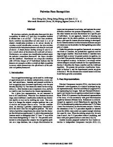
Scan path generation experiments Scan path generation experiments were carried out on face images, from a database collected by Cottrell & Metcalfe (1990). We used facial images of 35 people, with 8 expressions each (see Figure 2). We used Gabor filters with 8 orientations and 6 scales to calculate 48 element filter responses at each pixel. We computed the variance of the 8 filters at each scale separately. Figure 3 shows potential values at each scale converted to gray levels. The values of λ used are given across the top of the Figure. For the IF filter (Equation 5) and the recovery process (Equation 6), we tried the following parameters: α

(4)

When multiple scales and orientations are used, we get a feature vector of these responses for every point. This is basically the “Gabor jet” used by von der Malsburg and colleagues (Buhmann et al., 1991). We define the attentional field as the activity of units in a feature map. This activity, the attraction value for attention, is defined as the variance of the Gabor filter outputs over the multiple orientations at a particular resolution. We denote this V (κ, x~0 ). Note we assume a particular resolution of filter must be chosen based on the size of the object in the image for the purposes of attention selection. In our experiments here, we simply selected λ = 8. Thus, we model the low-level attentional attraction by the activity of the units in V . Then the scan path is generated as follows: 1. The point x~a , corresponding to the unit in the attentional field with the highest potential value is selected as the focus of attention point. 2. Once a point is visited, it is inhibited via a off-centeron-surround mask, given by:

∈

{0.1, 0.25, 0.5, 1.0}

β = 1 A = sR B = s ∈ δ

√

∈

3sR {0.5, 1.0, 2.0}

{0.02, 0.05, 0.10}

where R is 2σ/κ in Equation 1. A mechanism of controlling the scale to be used is beyond the scope of this paper. In the following experiments, we use the fourth scale from the left in Figure 3, that is, λ = 8, for the scan path generating experiments. Following the method outlined above, we generate a sequence of points. When a sequence of points longer than 5 is repeated, we define that as a scan path. Thus, if no sequence of attention points is repeated, no scan path is detected. We allow some jitter: An attention point within 4 pixels of a previous attention point is regarded as the same attention point.

Experimental results and discussion

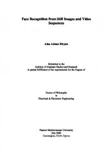
As described above, faces of 35 people are sampled. 8 kinds of expressions are used for each person, resulting in 0 |2 0 |2 ~ ~ 280 face images. An example is shown in Figure 4. The | x ~ − x | x ~ − x a a IF (x~a , x~0 ) = (1+α exp( ))(1−β exp( )) upper–left corner image shows a generated scan path. 2 2 A B (5) The first image to its right is the original potential field

Figure 2: Example faces (from Cottrell & Metcalfe, 1990). used for selecting the first point. One can clearly see the inhibition and recovery of points in this potential field as they are scanned. Each subsequent image shows the current selected attention point along with the previous nine points. The image sequence proceeds from left to right and top to bottom. As noted above, we did a parameter search through three parameters of our inhibitory surround (width, decay of inhibition, and strength). Table 1 shows the fraction of images that resulted in scan paths by our criterion for the various values of α, s, and δ. Table 1. Percent of scan path generation α 0.10 0.25 0.50 1.00 s δ 0.5 0.02 0.0% 0.0% 0.0% 0.0% 0.5 0.05 0.0% 0.0% 0.0% 0.0% 0.5 0.10 0.0% 0.0% 1.1% 6.4% 1.0 0.02 0.0% 0.0% 0.0% 0.0% 1.0 0.05 0.0% 0.0% 0.0% 0.4% 1.0 0.10 2.5% 4.6% 6.4% 20.7% 2.0 0.02 16.4% 16.4% 18.2% 18.2% 2.0 0.05 43.6% 44.3% 41.1% 45.4% 2.0 0.10 73.6% 73.2% 76.1% 82.9% In the case when the range parameter for facilitation and inhibition, s is 0.5, few scan paths are generated. An attention point is selected, potential values near the point are facilitated, and attention does not move to points far from the previous point. When the parameter s is larger,

more scan paths are generated. When the time constant parameter δ is too small, it takes too long for inhibited potential values recover. Therefore, it is hard for attention to return to previously selected points. The larger parameter α is, smaller the width of the ring area where potentials are facilitated. That is, the distance between two successive attention points stabilizes. However, scan path generation does not depend very strongly on this parameter. When s = 2.0 and δ = 0.1, scan paths are generated for about 73% to 83% of face images. The average length of scan paths in this case is about 40. Examples of scan paths which are generated from face images of 15 people are shown in Figure 5. The name of an image is of the form id.sex.emotion, followed by a number indicating the length of the scan path. Note this is the total number of points in the path, since many points are repeated. For five out of the thirty five images, no scan path is generated (marked N50).

Face recognition using scan paths We now employ our scan paths for object recognition. Our approach is as follows: We first changed the inhibition parameters slightly in order to get a wider range of points from a face. Then, we use one image of each of the 35 subjects in order to obtain a stored scan path. We allowed ourselves the freedom to alter parameters if the settings did not result in a scan path, until we did have a scan path for every face. Obviously in the future we would prefer to use an adaptive algorithm for this.

Figure 3: Variance of Gabor jets at difference scales. When storing these scan paths, in order to reduce processing time, we only stored the top 20 unique points, and the vectors to the next point. Now for recognition, when we encounter a new face, we first extract the top K attention points. We then compare these to the first attention points in the stored images. We do this by computing the cosine of the angle of the vectors of Gabor filter outputs subtracted from 1 to give a dissimilarity value. Using a threshold ξ, we accept as possible recognition candidates all stored images whose dissimilarity is less than ξ. Then, for each possible recognition candidate, we search the input image for the best fit of the next point along the stored scan path. To do this, we recall the stored trajectory from the matched point, and find the best match to the next point within a 5x5 patch of pixels centered at the end of that vector in the input image. If the summed dissimilarities for all points along the trajectory are less than ξ, we have a match. If more than one stored scan path matches, we take the lowest one. The 280 face images that were used for scan path generation simulation were used for the face recognition experiments. One face image for an individual is used in the face memorizing phase. Other 7 faces for an individual are used for recognition test. The number of recognition target categories is 35, one for each individual. The results of this procedure for various values of the threshold parameter are shown in Table 2. In Table 2 we also show the effect of varying the number of Gabor filter resolutions used, from all 6 (48 total filter values) down to 1. We see that for this task, it is important to use the whole Gabor jet for matching points.

Table 2. Face recognition rates using scan paths No. of thresh Hit Reject Error λ’s ξ rate (%) rate (%) rate (%) 6 1.2 96.7 2.4 0.8 6 1.0 94.3 4.9 0.8 6 0.8 90.2 9.8 0.0 5 1.0 93.1 5.7 1.2 5 0.8 85.7 13.9 0.4 5 0.6 70.6 29.4 0.0 3 0.8 89.0 9.4 1.6 3 0.6 81.2 18.0 0.8 3 0.4 60.4 39.6 0.0 1 0.6 82.9 1.2 15.9 1 0.4 79.2 14.7 6.1 1 0.2 56.3 43.7 0.0

Conclusion In this paper, we explored a model of scan path generation based on an easily computed value of low-level features, i.e., the variance of a set of Gabor filters at various points in an image. We found that the scan paths generated by our algorithm qualitatively matched human scan paths. We also found that the scan paths were useful for recognition. Given stored scan paths, individuals may be recognized by matching the stored features to those found by traveling along the trajectory given by the stored scan paths. This technique is relatively insensitive to changes of facial expression. Like von der Malsburg’s work, we find that one image is enough for recognition. Unlike von der Malsburg, we are able to recognize an image without a relaxation process, and we use only the top 20 “most exciting” feature points to do it. However, we have not yet explored recognition of

Figure 4: Generation of a scan path. See text for explanation. multiple orientations with our model.

Acknowledgements This work was performed while the first author was a Visiting Scholar in the lab of the second author, funded by NEC Corp, in 1990-1991. We thank the reviewers for Cognitive Science 1995 for being more open than the 1993 reviewers to the novelty of our work.

References . Ahmad and S. Omohundro (1990) A network for extracting the locations of point clusters using selective attention. International Computer Science Institute TR#90-011.

.Gabor (1946) Theory of communication, J. IEE 93, pp.429–457. .Koch & S. Ullman (1985) Shifts in selective visual attention: Towards the underlying neural circuitry. Human neurobiology 4, pp. 219–227. .A.Norman (1968) Toward a theory of memory and attention. Psychological review 75, pp.522-536. . Noton and L. Starks (1971) Eye Movements and Visual Perception, Scientific American 224, pp.34–43. .Noton (1971) Scanpaths in Eye Movements during Pattern Perception. Science 171, pp.308–311.

.Blum (1961) A model of the mind, Wiley: New York. . Buhmann, J. Lange, C. v.d.Malsburg, J.C. Vorbr¨ uggen and R.P. W¨ urtz (1991) Object Recognition with Gabor Functions in the Dynamic Link Architecture: Parallel Implementation on a Transputer Network. In B. Kosko, (Ed.), Neural Networks for Signal Processing. Englewood Cliffs, NJ: Prentice Hall , pp. 121–159. ottrell, G.W. & Metcalfe, J. (1991) EMPATH: Face, gender and emotion recognition using holons. In R.P. Lippman, J. Moody, & D.S. Touretzky (Eds.), Advances in neural information processing systems 3, pp. 564–571, San Mateo, CA: Morgan Kaufmann. .G. Daugman (1988) Complete discrete 2-D Gabor transforms by neural networks for image analysis and compression, IEEE trans. on Acoustics, speech, and signal process. 36. .A.Deutsch and D. Deutsch (1963) Attention: Some theoretical considerations. Psychological review 70, pp.80–90.

.H. Phaf, A.H.C. Van der Heijden, and P.T.W. Hudson (1990) SLAM: A Connectionist Model for Attention in Visual Selection Tasks. Cognitive psychology 22. .D. Rimey and C.M. Brown (1990) Selective Attention as Sequential Behavior: Modeling Eye movements with an Augmented Hidden Markov Model. U. of Rochester CS TR 327. . Treisman (1969) Strategies and models of selective attention, Psychological review 76, pp.242–299. . Treisman (1985) Preattentive processing in vision. Computer vision, graphics, and image processing 31, pp.156–177. . Ullman (1984) Visual routines. Cognition 18, pp:97– 159. .D.Whitehead and D.H. Ballard (1992) Learning to Perceive and act. U. of Rochester, Computer Science Technical Report.

Figure 5: Example scan paths. eremy Wolfe (1994) Guided Search 2.0 A revised model of visual search. Psychonomic Bull. & Rev. 1 2:202– 238.