A Modified Sensor Network Boundary Discovery

International Journal of Computer Applications (0975 – 8887) Volume 72– No.16, June 2013

A Modified Sensor Network Boundary Discovery Algorithm S.S.Riaz Ahamed

T.Anand

S. Ramakrishnan

AMIE.,MCA.,MPhil.,M.TechMA CM.,MIEEE.,Ph.D.,FIETE., Principal, Sathak Institute of Technology, Ramanathapuram , Tamilnadu, India.

M.E.,Ph.d Associate Professor

B.Sc. M.C.A Web Developer

Department of Computer Science and Engineering Madha Group Of Academic Institutions, Kundrathur, Chennai Tamilnadu, India.

ABSTRACT A WSN computer network using sensors is used in important application like environmental monitoring warning dangers to human lives. WSN‟s may have several problems related to topology construction, maintenance, and connectivity. The deployed Sensor devices may have critical resource constraints in terms of energy consumption. Also the algorithms need to be memory-efficient. Algorithmic issues arise in sensor deployment and coverage, routing, and fusion. Applications which rely on timely sensor updates on environments may have unpredictable results due to sensor inefficiencies. WSN applications may be in operation for months without wired power supplies, thus requiring to meet the delay requirements at minimum energy cost. Though various algorithms and protocols have been proposed for deploying sensors This paper proposes a new Algorithm CN Algorithm for WSNs and discusses WSNs. Future work includes the extension of the algorithm to detect the coverage boundary of the network or area covered by the sensor nodes inside a network.

General Terms Wireless Sensor Networks, Border Discovery.

Keywords WSN, routing, sensor network, WSN algorithm.

1. INTRODUCTION Wireless Sensor Networks (WSN) is a trend in modern networking. WSN‟s have revolutionized the networking world. A WSN is a computer network with spatially distributed individual devices using sensors. . Most sensor nodes are deployed in regions without infrastructure like placing a node by throwing it from an airplane. WSN applications are applied to areas where it is difficult to implement traditional networks. Applications can support digital delivery in rural areas or wildlife and habitat monitoring [1, 2]. A WSN sensor node is a small and cheap device used to monitor physical or environmental conditions co-operatively. WSN was originally developed for military operations. Advances in technology with enhanced data processing, wireless communication have also made use of sensor nodes and WSN‟s. Any WSN usually consists of hundreds or thousands of sensor nodes randomly deployed. The nodes are typically equipped with a wireless communication device, a small microcontroller and a battery.

WSN Research has attracted academicians and industrialists. WSN networks depend on the sensor nodes also called a tiny device. They capture and send data in a region. Wireless sensor network also provides an efficient way to connect physical environment and the web where the protocol is self organized for working cooperatively. The topology of a WSN may vary from a star network to A multi-hop wireless mesh network [3]. Research‟s have indicated the development of many protocols but wireless link reliability is considered in recent researches [4]. The data gathered from a WSN is generally stored as numerical data in a central base station. Algorithms remove or reduce redundant information in nodes for reducing communication costs. WSN‟s pose research challenges ranging from hardware to architectural issues, programming, security concerns, algorithms, deployment, operation and management. WSN also poses a number of unique challenges different from traditional wireless ad-hoc networks.

2. ISSUES IN WSN There are several Issues in WSN including Reliability, Realtime deployment, Mobility of nodes and many more. Sensor nodes are also redeployed due to many reasons like malfunctioning nodes. Wireless Sensor networks with tiny sensor nodes that sense events and process the data using wireless communication capabilities are thrown randomly in a mass. After deployment topology is affected due to variations in sensor nodes' location or reachability or depleting sensor energy. Sensors decisions based on the knowledge obtained from neighboring nodes is another fundamental problem during the development of a sensor network. In a centralized deployment, scalability is a problem due to the number of sensors. In random deployment the indefinite landing positions of the sensors is a potential problem, since the density of the nodes may not be uniform, leaving some areas uncovered. Since messages travel between nodes it is important to have reliability on links and lack of which decreases the probability of a message being in transit. MANET routing algorithms like DSR, AODV do not perform well in a WSN because they send a discovery message from a source to a destination and use the less reliable acknowledgements. To save power many WSN‟s place nodes into sleep states and a node cannot choose a sleeping node as the next hop or until it finds an active node. Moreover, the degree of uncertainty in a WSN makes it difficult to develop routing algorithms with guaranteed delivery. The energy consumption models established that the energy consumed by 1

International Journal of Computer Applications (0975 – 8887) Volume 72– No.16, June 2013 transmitting a unit of data was the same for each node though it was hard to evaluate based on elusory communication distance measurements. The life of a network is increased by putting sensors not needed to provide coverage to sleep and awaken these sleeping sensors when needed. A sleeping node would wake up after its sleep timer expired and broadcast a probing signal. Power-aware routing have been investigated in several previous works.

3. ALGORITHMS FOR WSN’S In a WSN sensor Deployment and Coverage, the sensors are deployed to monitor a region as a set of points. Sensors in hostile environments are placed by simply scattering in large numbers over the monitoring region expecting they survive the air drop and adequately monitor the target region.WSN Algorithms can be categorized as either centralized or distributed. Since a WSN requires limited memory while computing and communication capability in sensors, distributed algorithms focus on a localized nearest neighbor information. Deterministic sensor deployment is used when site selection is possible and deployment is nondeterministic when site selection is not possible. The deployed collection of sensors need to form a connected network, since it is easy to check if the collection covers the target region. Zhang and Lou establish the necessary and sufficient condition for coverage to imply connectivity in Theorem 1 [5]. Theorem 1: Assuming the sensor density is finite c ≥ 2r is a necessary and sufficient condition for coverage to imply connectivity, Where r is the sensor‟s sensing range and c the communication range.

3.1 Greedy Algorithm Kar and Banerjee [6] examined the deployment of least number of homogeneous sensors to cover an area with a connected sensor network with the assumption that the sensing range equaled the communication range (i.e., r = c). The Greedy algorithm uses at most 7.26 times the minimum number of sensors needed to cover the given point set and covers all of the given points as a connected network.

3.2 Unicast Algorithms A unicast message is sent from a source s to a destination t. Singh, Woo and Raghavendra [7] proposed a selection in the routing path for a sensor transmission using a minimumenergy path from source s to Destination t. Aslam, Li and Rus [8] proposed the max-min zPmin-path algorithm to select unicast routes. Their algorithm selected a unicast path using z ∗ Pmin energy, where z is a parameter and Pmin, the energy required by the unicast path. All possible values for the residual energy fraction of node u is obtained by computing (ce(u)−w(u, v) ∗ l)/ie(u), where l is the message length, ce(u) the current energy at a node u, (u) the initial energy at u, and w(u, v), the energy needed to send a unit-length message along the edge (u, v). This computes all vertices v adjacent to u. Hence the union, L, of the values taken from u gives the possible values for the minimum residual-energy in any unicast path. In the CMAX algorithm, the weight of every edge (u, v) is changed from w(u, v) to w(u, v) * (λα(u) − 1). The shortest path P (source-to-destination) is determined in a resulting graph and for length more than σ, the unicast is rejected else the unicast works on the path P. The MRPC lifetime-maximization algorithm proposed by Misra and Banerjee [9] is based on the capacity, c(u, v) of edge (u, v) and defined as ce(u)/w(u, v). The lifetime of the path P life(P) is the minimum edge capacity on the path.

3.3 Clustering Algorithms WSN applications require a scalable architecture with a defined management. WSN environments need to be energy savers implying the designing of energy-aware algorithms an important factor. Grouping sensor nodes into clusters achieves the objectives with a leader called the cluster-head (CH). Clustering techniques may vary depending on the node deployment, network architecture and operation model. A CH may be a pre-assigned sensor node, richer in resources or elected by other sensors in a cluster. In addition to supporting network scalability, clustering has many advantages. It can localize the route within a cluster reducing the size of the routing table stored [10]. Clustering can also conserve communication bandwidth by interactions between CHs, avoiding redundant messages exchanges between sensor nodes [11]. Sensors connected with CHs do not get affected by changes at the inter-CH tier [12]. The CH can also be used to implement management strategies and prolong the battery life of individual sensors and increased network lifetime [11]. CH can aggregate the data collected in the cluster and decrease the number of relayed packets [13]. The linked cluster algorithm (LCA) [14] is one of the earliest algorithm in clustering of wireless networks with a focus on forming an efficient network topology capable of handling mobility of nodes. Since a CH is directly connected to the nodes in its cluster, it is geared for maximum network connectivity. The LCA algorithm assumes that the nodes are synchronized and have a time-based access. A node is assigned the slot in the frame that matches its ID. Initially, Each node broadcasts its ID and listens to Cluster properties of other nodes. Next a node broadcasts to know its 1-hop and 2-hop neighbors. A CH has the highest ID among its neighbors. LCA yields excessive number of clusters. The random competition based clustering (RCC) designed for mobile ad hoc networks [15] is also applicable to WSN‟s. RCC‟s main focus is cluster stability to support mobile nodes. In the RCC algorithm any node can „govern‟ the rest of the nodes if it is the first to claim being a CH. After the claim broadcasted by the first node, the neighboring nodes join its cluster as member. The CH broadcasts a claim packet periodically. Time delays between broadcasting a claim packet and receiving it, can possibly create a conflict and to avoid such a problem RCC explicitly employs a random timer and uses the node ID for arbitration. Each node in the network resets its random time value every time before broadcasting its CH claim packet. During this random time if it receives a broadcast message carrying CH claim packet from another node, it simply ceases the transmission of its CH claim. RCC resolves concurrent broadcast problems by using the node ID. When the conflict persists node having a lower ID becomes the CH. RCC is found to be more stable than conventional clustering schemes. Banerjee and Khuller demonstrated a multi-tier hierarchical clustering [16]. Figure 1 illustrates the concept of hierarchy in clusters. A cluster‟s properties like cluster size, degree of overlap, are used for management and scalability of the hierarchy. Any node can initiate the cluster formation process where the Initiator with least node ID takes precedence when multiple nodes start cluster formation process at the same time. The algorithm proceeds in two phases: Tree discovery and Cluster formation. The tree discovery is a distributed formation of a Breadth-First-Search (BFS) tree rooted from the initiator node. Broadcast signal carry the information such as source ID, parent ID, root ID, and sub-tree size. Each node, u, broadcasts a signal for p units of time, carrying information on its shortest hop-distance to the root, r. A node v chooses a neighbor u to be its parent and updates its hop-distance to the root, if the route through u is shorter. Every node gets 2

International Journal of Computer Applications (0975 – 8887) Volume 72– No.16, June 2013 updated when its children update their sub-tree size. The cluster formation starts when a sub-tree crosses the size parameter, k and the node initiates cluster formation.

 

Communications are bidirectional and symmetric. Nodes can determine its distance from neighbors.

4.2 Notations And Definitions    

n is the number nodes in a sensor network G = (V,E) is the Graph where n = |V | set of nodes in the network E is the set of undirected edges e(i, j)



i, j ∈ V node j is in node I‟s communication range



Figure 1 Three Layer Cluster Hierarchy (Figure is redrawn from [16]) Leach Low Energy Adaptive Clustering Hierarchical Protocol (LEACH), is a clustering-based protocol that minimizes energy dissipation in WSN‟s [17]. LEACH randomly selects sensor nodes as cluster-heads for high energy dissipation. LEACH protocol has many rounds and each round has two phases, a setup phase and steady state phase. In the set up phase it provides cluster formation in an adaptive manner and in the steady state transfers data. The duration of the steady phase is longer than the duration of the set-up phase to minimize overheads. During the set-up phase, a sensor node chooses a random number between 0 and 1 and when this random number is lesser than the threshold value, the sensor node becomes a cluster-head. P is the desired percentage to become a cluster head, r is the current round, and G is the set of nodes that have not being selected as a cluster-head in the last 1=P rounds. After the cluster-heads are selected, they advertise to all sensor nodes that they are the new clusterheads. Once the sensor nodes receive the advertisement, they determine the cluster that they want to belong to based on the signal strength of the advertisement. The sensor nodes inform the appropriate cluster-heads that they will be a member of the cluster. The cluster-heads assign the time on which the sensor nodes can send data to the cluster-heads based on a Time Division Multiple Access (TDMA) approach. During the steady phase, the sensor nodes can begin sensing and transmitting data to the cluster-heads. They also combine data from the nodes and the cluster before sending these data to the base station.

4. ENERGY EFFICACY COMPUTING WSN systems require a random deployment of sensor nodes over a large target area with detection of activities within a boundary. The sensors need to be capable of detecting and identifying any object that enters or leaves the monitored area. It is challenging but necessary to identify the boundary nodes ( nodes which represent the perimeter of the target area). WSN systems are generally dynamic in nature, since they keep evolving. Nodes may fail due to power shortage or displacement due to a natural phenomenon or when nodes are redeployed. This section introduces a modified algorithm for detecting the boundary nodes of a WSN. It relies on communication between nodes and its neighboring nodes, making it applicable to large-scale WSNs.

4.1 Assumptions   

Nodes are homogenous with a unique global ID. The network density is 2 to 4 neighbors. Network has no communication holes.

Let p ∈ V be a node in the network Define N2(p) to be the set of all the nodes that are within 2 hops from node p. Formally, N2(p) = {i : i ∈ V, d(p, i) ≤ 2}, where d(p, i) represents the distance between nodes p and i. Thus, N2(p) represents the 2nd order closed neighborhood of p in G. The set N1(p), or simply N(p), contains all nodes that are within the communication range of node p. Formally, N(p) = {i : i ∈ V, (p, i) ∈ E}. Interior Node: A node p ∈ V is said to be an interior node if there ∃ at least three nodes a, b ∈ V such that a, b ∈ N(p) and the nodes a, b forms a line that encloses the node p. Boundary Node: A node p ∈ V is said to be a boundary node if p is not an interior node. Define B to be the set of boundary nodes in the network; and I to be the set of interior, i.e. non-boundary, nodes in the network. Network Boundary: The imaginary line that connects the boundary nodes of the sensor network is defined as a network boundary. The network boundary defines the perimeter of the entire network.

4.3 Problem Identification Given a graph G =(V,E), where nodes of G are in a two dimensional space. For a node p ∈ V , determine if there exists a set S such that S ⊂ N(p), and |S| 2, where with at least two nodes a, b ∈ S that enclose the node p in a line.

4.4 Choose Neighbors (CN) Algorithm Three neighbors A, B and C of node P are chosen because each node will be have more than three neighbors. Node P may will be interior or exterior node depending on the three neighboring nodes. Let the neighbors A, B and C be the three neighbors of the P, then P is an interior node as it can be enclosed inside the ΔABC. But in case P is an exterior to ΔABD algorithm selects four neighbors, A, B, C and D, of a node P. The node P is detected as an interior node if it is either inside the ΔABC or ΔABD. The algorithm tries to discover neighbors close to the given node. First, a node A closest to the given node P is found, then a node B is searched (on the opposite side, to side of A to P), a third node C, is searched which is equidistant from A and B, but at a minimum distance from P (anywhere inside the search space ) and finally P could not be enclosed inside ΔABC. P could be detected as an exterior node and node D, is searched equidistant from A and B, and at a maximum distance from C. When no node D is found node P is not inside ΔABC, then node P is a boundary node.

4.5 The CN Algorithm Input: Node P. Output: Four nodes A, B, C,D of P 1. Find a node from N(P) which at the minimum distance from P. Name it as node A. 2. SearchRadius = dPA; 3. WHILE(CommunicationRange _= SearchRadius) FOR all the nodes within SearchRadius of P

3

International Journal of Computer Applications (0975 – 8887) Volume 72– No.16, June 2013 Find a node B, such that it is in both N(P) and N(A), and distance dAB is maximum. ROF IF node B is found EXIT WHILE ELSE SearchRadious++; END-WHILE 4. Find a node C such that it is in N(A), N(B) and N(P), and |dAC − dBC| is minimum and dPC is minimum. 5. Find a point D such that, D is in N(A), N(B), N(C), N(P) and |dAD − dBC| is minimum and dDC is maximum and dDC > dDP and dDC > dPC 6. IF (InteriorPoint (P,A,B,C)) RETURN ‟P is an interior point.‟ ELSEIF (InteriorPoint (P,A,B,D)) RETURN ‟P is an interior point.‟ ELSE RETURN ‟P is a boundary point‟.

5. RESULTS This section describes the simulations performed to evaluate algorithms and analysis of the results obtained. MATLAB was used to simulate algorithms with the assumption that the communication range of all the nodes in the network was of fixed radius and all the communication channels symmetric. For our simulation, the area of deployment was divided into unit grids with two types of sensor network deployment namely grid deployment and random deployment. In grid deployment, the nodes were placed exactly at the grid points. Random deployment deploys the sensors randomly inside one unit grid. It was assumed that each node in the network knew all its one-hop neighbors and its distance to them.. Each node could locally query all its one-hop neighbors and acquire the one-hop neighbor list from each of them. Three different evaluation parameters were considered for the simulationnumber of nodes, node communication range and sensor network deployment. Each scenario was simulated a number of times, With temperature as the monitoring object. Although the nodes sensed the temperature continuously along the time, data are sent only when the minimum or the maximum value collected differed 2% from the last data sent, inducing the event-driven property to the sensing application. In order to simulate the temperature behavior of the environment, random numbers were generated following a normal distribution with a standard deviation of 1 from an average temperature of 25 Degrees C.

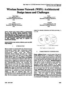
Figure 2 Delivery rate of messages in WSN. Figure 2 shows the delivery rate for sensing application and management messages. It is observed that for scenarios 1 and 2 the delivery rate for management messages and

application messages were similar. The result exhibited in Figure 2 concerns the delivery rate of application messages. The introduction of management had little impact on the sensing application.

Figure 3 Number of messages transmitted by nodes in WSN. Figure 3 shows the traffic of messages in the WSN. The management contributes a small increase (18.49%) in the WSN traffic when they are event driven. However, the number of messages sent almost doubled (increase of 93.33%) when management with detection is concerned.. Figure 4 shows the energy consumption of common-nodes and clusterheads for all scenarios 1, 2, and 3. It was observed that, the energy consumption increased with management in 18% for cluster heads and 29.45% for nodes. But when the detection mechanism was taken into account, management caused an increase of 101.2% and 129.45% in the energy consumption for cluster-heads and nodes, respectively. This result was expected since the act of transmitting and receiving messages are the most determinant activities for energy consumption according to the simulated energy model.

Figure 4 Energy consumption of nodes in the WSN.

6. CONCLUSION Wireless Sensor Networks represent a new frontier in the development of technologies. Research shows there are several problems needing investigation like border protection or disaster management. These applications a large number of sensors require careful architecture and management strategies. Grouping nodes into clusters has been a popular approach for in WSNs. Significant attention has been paid to clustering strategies and algorithms.. The sensors need to identify any object that enters or leaves the monitored area. It is challenging but necessary to identify nodes which represent the perimeter of the area. This dissertation has proposed an algorithm that can be used to discover the boundary nodes of a randomly deployed WSN in the shortest possible path. This submission has proposed a new baseline for a fast protocol in WSN to save energy. Future work includes the extension of the algorithm to detect the coverage boundary of the network, encompassing the areas that could be monitored or covered by the sensor nodes inside the network.

4

International Journal of Computer Applications (0975 – 8887) Volume 72– No.16, June 2013

7. REFERENCES [1] I.F. Akyildiz, W. Su, Y. Sankarasubramaniam, and E.Cayirci, “Wireless sensor networks: A survey,” Computer Networks, vol. 38, no. 4, pp. 393–442, December 2002, [2] M. Kuorilehto, M. Hannikainen, and T.D. Hamalainen, “A survey of application distribution in wireless sensor networks,” EURASIP Journal on Wireless Communications and Networking, vol. 2005, no. 5, pp. 774–788, March 2005. [3] Dargie, W. and Poellabauer, C., "Fundamentals of wireless sensor networks: theory and practice", John Wiley and Sons, 2010 ISBN 978-0-470-99765-9, pp. 168–183, 191– 192. [4] Matischek: Real-Time Communication MAC Protocols for Wireless Sensor Networks, 2012, ISBN 978-3-83006349-0 [5] H. Zhang and J. Hou, Maintaining sensing coverage and connectivity in large sensor networks, Technical Report UIUC, UIUCDCS-R-2003-2351, 2003. [6] K. Kar and S. Banerjee, Node placement for connected coverage in sensor networks, Proc WiOpt 2003: Modeling and Optimization in Mobile, Ad Hoc and Wireless Networks, 2003.

[10] K. Akkaya, M. Younis, A survey on routing protocols for wireless sensor networks, Elsevier Journal of Ad Hoc Networks 3 (3) (2005) 325–349. [11]

M. Younis, M. Youssef, K. Arisha, Energy-aware management in cluster-based sensor networks, Computer Networks 43 (5) (2003) 649–668.

[12]

Y.T. Hou, Y. Shi, H.D. Sherali, On energy provisioning and relay node placement for wireless sensor networks, IEEE Transactions on Wireless Communications (2005) 2579–2590

[13]

K. Dasgupta, K. Kalpakis, P. Namjoshi, An efficient clustering based heuristic for data gathering and aggregation in sensor networks, in: Proceedings of the IEEE Wireless Communications and Networking Conference (WCNC, 2003), New Orleans,

[14]

D.J. Baker, A. Ephremides, The architectural organization of a mobile radio network via a distributed algorithm, IEEE Transactions on Communications, COM-29 (11) (1981) 1694– 1701.

[15] K. Xu, M. Gerla, A heterogeneous routing protocol based on a new stable clustering scheme, in: Proceeding of IEEE Military Communications Conference (MILCOM 2002), Anaheim, CA, October 2002. [16]

S. Banerjee, S. Khuller, A clustering scheme for hierarchical control in multi-hop wireless networks, in: Proceedings of 20th Joint Conference of the IEEE Computer and Communications Societies (INFOCOM‟ 01), Anchorage, AK, April 2001

[17]

W. Heinzelman, J. Kulik, and H. Balakrishnan, Adaptive Protocols for Information Dissemination in Wireless Sensor Networks, Proceedings of the 5th Annual ACM/IEEE International Conference on Mobile Computing and Networking (MobiCom‟99), Seattle, WA, August 1999.

[7] S. Singh, M.Woo, and C. Raghavendra, Power-aware routing in mobile ad hoc networks, ACM/IEEE MOBICOM, 1998. [8] J. Aslam, Q. Li and R. Rus, Three power-aware routing algorithms for sensor netowrk, Wireless Communications and Mobile Computing, 3, 2003, 187208. [9] A. Misra and S. Banerjee, MRPC: maximizing network lifetime for reliable routing in wireless,,IEEE Wireless Communications and Networking Conference (WCNC), 2002.

5 IJCATM : www.ijcaonline.org