A Multidimensional Branch-and-Prune Method for Interval Global ...

A Multidimensional Branch-and-Prune Method for Interval Global Optimization ∗ Tam´as Vink´o ([email protected]) Reseacrh Group on Artificial Intelligence of the Hungarian Academy of Sciences and University of Szeged, H-6720 Szeged, Aradi v´ertan´ uk tere 1., Hungary

Dietmar Ratz ([email protected]) Department of Applied Informatics and Formal Descriptions, University of Karlsruhe, Karlsruhe, Germany Abstract. In this paper a new multidimensional extension of the recently developed one-dimensional enclosure method called kite is given for interval global optimization. A more sophisticated version of the pruning technique based on the kite method is introduced. By the new componentwise approach all the one-dimensional theoretical results and procedures can be used in the higher dimensional case. The possibilities in the implementation of the new algorithm together with numerical results on 40 standard test problems are presented. Keywords: Interval methods, global optimization, inclusion function, pruning, kite AMS classification: 90C30, 65K05

1. Introduction In a recent paper a new inclusion function called kite enclosure has been developed and investigated for global optimization for the onedimensional case [12]. The aim of the present paper is to give an extension of those results for the multidimensional problems. Consider the problem of finding all solutions x∗ of min f (x)

(1)

x∈X

where the objective function f : D ⊆ Rn → R is continuously differentiable and X ⊆ D is the search box representing bound constraints for x. We wish to find the set of all global minimizers x∗ and the global minimum value f (x∗ ). With interval global optimization algorithms based on branch-and-bound methods [3, 4, 9] we can provide guaranteed and reliable solutions for the problem (1). In the following real numbers are denoted by lower case letters (a, b, . . .) and real bounded and closed n-dimensional intervals by capital letters (X, Y, . . .). The set of compact intervals is denoted by I := ∗

This work has been supported by the grant OTKA T 034350 c 2005 Kluwer Academic Publishers. Printed in the Netherlands. °

bnp.tex; 25/02/2005; 12:45; p.1

2

A Branch-and-Prune Method for Optimization

{[a, b] | a ≤ b; a, b ∈ R}. In general the lower and the upper bounds of an interval X = X1 × . . . × Xn are denoted by X and X, respectively. The range of the function f on X is denoted by f (X). We call a function F : In → I an inclusion function of f in X if x ∈ Y implies f (x) ∈ F (Y ) for all Y ∈ I(D) ⊆ In , where I(D) stands for all intervals in D. Applying automatic differentiation [2, 4, 6] we are able to compute inclusion functions for the derivatives without additional human interaction. An enclosure of the gradient vector f 0 (y) is denoted by F 0 (Y ), while the ith component of this vector by Fi0 (Y ) = [Li , Ui ]. For all i = 1, . . . , n the inequality Li Ui < 0 is supposed in this work. The detailed forms of the branch and bound algorithm used in this paper can be found in [2, 3, 4, 9]. Here a new accelerating tool is investigated which is based on the pruning possibilities of the onedimensional kite method. 2. Componentwise extension of the kite enclosure method In the one-dimensional case the kite inclusion function is simply the simultaneous usage of the linear boundary value form [7] and the centered form [8] with a proper selection of the center point. For higher dimension the extension of the linear boundary value form exists (see [5] for details). The centered form is also available for multidimensional functions. However, the simultaneous usage of them is in general difficult to realize. In the following an effective and easier to implement way of the extension is given. In [11] the centered form and a pruning method based on slopes is developed for the multidimensional case in a componentwise manner. The extension of the kite enclosure together with the pruning effect is also possible in this way. In the following this approach is discussed. Let f : D ⊆ Rn → R and Y = Y1 × . . . × Yn ⊆ D. Let us define gi : Yi ⊆ R → I (i ∈ {1, . . . , n}) by gi (w) := f (Y1 , . . . Yi−1 , w, Yi+1 , . . . , Yn ), w ∈ Yi .

Using this one-dimensional interval valued function we are able to use the one-dimensional version of the kite enclosure method. If we have V ⊇ gi (Y i ), W ⊇ gi (Yi ) and Z ⊇ gi (ci ) where (ci ∈ Yi ), then the componentwise kite enclosure can be built up with the usage of the componentwise centered form, i.e. F CF (Y, c, i) = Z + Fi0 (Y )(Yi − ci ),

(ci ∈ Yi ),

and the componentwise linear boundary value form Ui V − L i W L i Ui F LBV F (Y, i) = + (Yi − Y i ) . Ui − L i Ui − L i

(2)

(3)

bnp.tex; 25/02/2005; 12:45; p.2

T. Vink´ o and D. Ratz

3

The simultaneous usage of the formulae (2) and (3) leads to the following result. THEOREM 1. Let F K (Y, c, i) = min{yR (c, i), yT (c, i)}, where c ∈ Y , Ui V − Li Z + Ui Li (ci − Y i ) , Ui − L i Ui Z − Li W + Ui Li (Yi − ci ) yT (c, i) = , Ui − L i

yR (c, i) =

Z ⊇ gi (ci ), V ⊇ gi (Y i ) and W ⊇ gi (Yi ), and i = 1, . . . , n. Then max{F LBV F (Y, i), F CF (Y, c, i)} ≤ F K (Y, c, i) ≤ f (Y )

(4)

hold for every i = 1, . . . n. Proof. One can proceed the proof of the Proposition 2 from [12] for all i = 1, . . . , n. 2 Note that Theorem 1 tells that the componentwise kite method is not worse than the componentwise centered form or the componentwise linear boundary value form (for the same component Yi of the interval Y ). In the formula (4) the parameter c can be set to be optimal. That is we can find the point c∗ such that F K (Y, c∗ , i) = max F K (Y, c, i) = max min{yR (c, i), yT (c, i)}. c∈Y

c∈Y

(5)

To obtain this optimal c∗ the Theorem 1 of [12] can be used for every coordinate direction. Note that here the value c∗ depends on the interval Y and the direction i, i.e. if i 6= j then the value c∗ (Y, i) is usually not equal to the value c∗ (Y, j). From [12] we know that the point c∗ (Y, i) is not always unique and it can be given as a solution of a nonlinear equation, which has the form αi gi (z) + βi = 0 (αi , βi , z ∈ R). In the implementation we usually do not compute the exact value of c∗ (Y, i), only an approximation of it is given using the same technique as in the one-dimensional case. For details see [12]. From the formula (4) or even from (5) a lower bound for f (X) can be obtained: the value max1≤i≤n F K (Y, c, i) is always less than or equal to f (Y ). However, the centered form or the multidimensional extension of the linear boundary value form can give a better (greater) lower bound for the range of the objective function in general. To compute a lower bound for the value f (Y ) with the componentwise kite inclusion 3n function evaluations (2 evaluations at the endpoints and 1 evaluation at

bnp.tex; 25/02/2005; 12:45; p.3

4

A Branch-and-Prune Method for Optimization

the centers) and one gradient evaluation are needed. Thus, the componentwise versions of the inclusion functions above are not recommended to be used in the interval global optimization algorithms. It is why this approach is used better in the construction of a new accelerating tool.

3. Componentwise pruning in higher dimension Using the computed value needed for the construction of the componentwise kite inclusion function a pruning method can be developed. The following theorem proves the correctness of the necessary formulae. THEOREM 2. Let Y ⊆ X ⊆ In be the current considered subinterval, c ∈ Y , F 0 (Y ) be an enclosure of the gradient of f (Y ), and f˜ be the current guaranteed upper bound for the global minimum value. If we have Z ⊇ gi (ci ), V ⊇ gi (Y i ) and W ⊇ gi (Yi ), f˜ − V , Li f˜ − Z ri = c i + , Li

pi = Y i +

f˜ − Z , Ui f˜ − W si = Y i + , Ui

qi = c i +

then for every i ∈ {1, . . . , n} the following statements hold. (a) If f˜ < min{V , W , Z} then all the global minimizer points of Y are contained in the intervals Y1 × . . . × Yi−1 × [pi , qi ] × Yi+1 × . . . × Yn and Y1 × . . . × Yi−1 × [ri , si ] × Yi+1 × . . . × Yn . (b) If W ≤ f˜ < min{V , Z} then all the global minimizer points of Y are contained in the intervals Y1 ×. . .×Yi−1 ×[pi , qi ]×Yi+1 ×. . .×Yn and Y1 × . . . × Yi−1 × [ri , Yi ] × Yi+1 × . . . × Yn . (c) If V ≤ f˜ < min{Z, W } then all the global minimizer points of Y are contained in the intervals Y1 ×. . .×Yi−1 ×[Y i , qi ]×Yi+1 ×. . .×Yn and Y1 × . . . × Yi−1 × [ri , si ] × Yi+1 × . . . × Yn . (d) If Z ≤ f˜ < min{V , W } then all the global minimizer points of Y are contained in the interval Y1 ×. . .×Yi−1 ×[pi , si ]×Yi+1 ×. . .×Yn . (e) If max{W , Z} ≤ f˜ < V then all the global minimizer points of Y are contained in the interval Y1 ×. . .×Yi−1 ×[pi , Yi ]×Yi+1 ×. . .×Yn . (f ) If max{V , Z} ≤ f˜ < W then all the global minimizer points of Y are contained in the intervals Y1 ×. . .×Yi−1 ×[Y i , si ]×Yi+1 ×. . .×Yn .

bnp.tex; 25/02/2005; 12:45; p.4

T. Vink´ o and D. Ratz

5

(g) If max{V , W } ≤ f˜ < Z then all the global minimizer points of Y are contained in the intervals Y1 ×. . .×Yi−1 ×[Y i , qi ]×Yi+1 ×. . .×Yn and Y1 × . . . × Yi−1 × [ri , Yi ] × Yi+1 × . . . × Yn . Proof. (a) Let x∗ ∈ Y ⊆ X be the global minimizer point and let i ∈ {1, . . . , n} be arbitrary but fixed. First, we have to show that pi ≤ x∗i holds. Since f˜ < V is supposed and V ≤ f (x∗ ) then x∗i 6= Y i . From the inequalities Li ≤

f (x∗ ) − V f˜ − V ≤ ∗ ∗ xi − Y i xi − Y i

we have (x∗i − Y i )Li ≤ f˜ − V . Then since x∗ ≥

f˜ − V + Y i = pi Li

holds because Li < 0 was supposed. To prove that x∗i is not included in the open interval (qi , ri ) first we suppose that x∗i < ci holds. Then from Ui ≥

f (x∗ ) − Z x∗i − ci

we have Ui (x∗i − ci ) ≤ f (x∗ ) − z ≤ f˜ − Z. From these inequality x∗i ≤ ci +

f˜ − Z = qi Ui

holds. Now suppose that x∗i > ci . Then from Li ≤

f (x∗ ) − Z f˜ − Z ≤ ∗ ∗ xi − c i xi − c i

we have (x∗i − ci )Li ≤ f˜ − Z. Then x∗i ≥ ci +

f˜ − Z Li

holds because x∗i − ci > 0 and Li < 0 were supposed. The case x∗i = ci is not possible, because Z = gi (ci ) > f˜ was supposed and f˜ ≥ f (x∗ ). Finally, from f˜ − W f (x∗ ) − W ≥ Ui ≥ x∗i − Yi x∗i − Yi

bnp.tex; 25/02/2005; 12:45; p.5

6

A Branch-and-Prune Method for Optimization

we have (x∗i − Yi )Ui ≤ f˜ − W . Then x∗i ≤ Yi +

f˜ − W Ui

holds because Ui > 0 by our earlier assumption. With this we completed the proof of the case (a). The proof of cases (b)–(g) are similar to the case (a) thus we have omitted them. 2

Based on the Theorem 2 we can conclude that in any case if Yi = [Y i , Yi ] and ((pi > Y i ) ∧ (si < Y i )) or ((qi < Y i ) ∧ (ri > Yi )) then the whole subinterval Y can be rejected: it does not contain any global minimizer points. 4. Proposed algorithm Now we give the algorithmic description of the new branch-and-prune global optimization method based on the above results. Step A Let X be the starting interval. Compute F (X), F 0 (X), initialize WorkList = {(X, F (X), F 0 (X))}, ResultList = {}, and the guaranteed upper bound f˜ = F (c) for the global minimum value. Step B While WorkList is not empty do the following steps. Step C Get (Y, F (Y ), F 0 (Y )) from the WorkList and for every coordinate direction of Y do the following steps. Step C.1 Compute the componentwise kite enclosure for the ith coordinate. Step C.2 Apply the pruning method based on the kite for the ith coordinate. Step D For the subintervals Ui (i = 1 . . . m ≤ n + 1) produced by the pruning do the following steps. Step D.1 Compute F (Ui ), F 0 (Ui ). Apply the monotonicity and the midpoint tests. Step D.2 Compute the centered form for Ui (and improve f˜ if it is possible). Step D.3 If the stopping criterion holds for the current interval then put it to the ResultList else put it (together with the values F (Ui ), F 0 (Ui )) to the WorkList.

bnp.tex; 25/02/2005; 12:45; p.6

T. Vink´ o and D. Ratz

7

Step E Go back to Step B. First of all it must be emphasized that in this new algorithm the componentwise kite enclosure is used as a pruning step (i.e. an accelerator) and not only as an inclusion function. To obtain a (possibly) better enclosure of the objective function on the current subinterval the original centered form is used (in Step D.2). This is done so since the centered form gives usually a better (higher) lower bound than the componentwise kite method. However, in the Step C the information needed for the kite enclosure could be used to update the value f˜. Also, the candidate subinterval Y can be rejected if the inequality f˜ < F K (Y, c, i) (i.e. a range test) is fulfilled. In the Step C.2 a special splitting technique is used which was introduced in [10]. This performs one component step according to the following scheme: 1. Let V, W ⊆ Yi the intervals produced by the pruning step. 2. If W = V = ∅, then stop (there is no solution in Y ). 3. If V 6= ∅, then set Yi := V and store Y. 4. Set Yi := W and continue with next i. With this method the pruning procedure produces at most n + 1 subintervals. If pruning is possible in an iteration step, then the inclusion of the derivative is not computed in the next iteration (which deals with the previously shrunk interval). Note that the Step C performs a bisection if no pruning is possible. In Step C it is not necessary to compute Yi in the fixed order i = 1, . . . , n. One can use a sorted index vector to obtain different orders of the components. In our experience we have tried to use sorted index vectors generated by interval branching rules from A to D [1]. We have found that the best choice is the rule C based on the maximization of the merit function D(i) = w(Fi0 (Y )(Yi − mid(Yi ))),

(6)

where w(X) and mid(X) denote the width and the midpoint of the interval X, respectively. The new index vector t = (t1 , . . . , tn ) with tk ∈ {1, . . . , n} and ti 6= tj for i 6= j, satisfies D(tk ) ≥ D(tk+1 ), k = 1, . . . , n − 1. According to our considerations above we can state that using the proposed algorithm we cannot loose global minimizer points which are in the starting interval X. In the pruning step for a given interval Y

bnp.tex; 25/02/2005; 12:45; p.7

8

A Branch-and-Prune Method for Optimization

if the value m is equal to zero then there is no global (with respect to X) minimizer of f in Y .

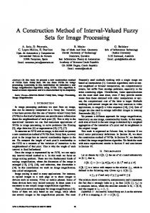
5. Numerical results This section deals with the discussion of the numerical results based on the componentwise realization of the multidimensional kite enclosure method and its pruning technique. The goal of the test is to demonstrate the effect and the behavior of the new accelerating tool compared to the traditional algorithm. The implementation of the algorithm given in the Section 4 has been done on a Pentium III, 1GHz computer under Linux operating system and in the environment of the C++ Toolbox for Verified Computing [2]. For the comparison the new algorithm was used without the Step C and in Step D the value m was set to be 2 (i.e. only bisection was used). In the computational experiments 40 standard test functions were taken from the literature. The stopping criterion was fulfilled when the maximal width of the current subinterval was smaller than 10−6 (except for the problems GP, Sch27, Sch214, G7, R5, R6, R7, R8, EX2 where this number was 10−2 .) Our numerical experience shows that in the computation of the componentwise kite enclosure using the formula (5) the resulted intervals gi (Y i ), gi (ci ), gi (Yi ) could be very large. In this case the pruning usually cannot be used because of that large overestimations. For this reason the algorithm leaves the pruning step (Step C) and do a bisection if one of the width of the intervals gi (Y i ), gi (ci ), gi (Yi ) is greater than a specified heuristic parameter. In our tests this parameter was set to be max{D(t1 ), 100}, where D is the merit function defined in (6). Using this modification the total computational effort can be reduced. Both algorithms were able to solve all the test problems. The numerical results are summarized in Table I. The given efficiency indicators are the number of the function evaluations (F-eval), the number of the derivative evaluations (D-eval), the maximal list length necessary (MLL) and the CPU time in seconds (CPUt). In the last but one row Σ denotes the sum of the given efficiency indicators followed by the relative compound indicator for the new method compared to the old one as per cents. The last row contains the average of the percentages (AoP) for the respective columns. Summarizing the results we can conclude that the number of function evaluations were larger for 24 test functions for the new method. It is understandable since the construction of the componentwise kite needs more function evaluations at the borders of the considered subin-

bnp.tex; 25/02/2005; 12:45; p.8

9

T. Vink´ o and D. Ratz

Table I. Numerical results of the basic and the kite pruning algorithm. Problem name dim. S5 S7 S10 H3 H6 GP SHCB THCB BR RB RB5 L3 L5 L8 L9 L10 L11 L12 L13 L14 L15 L16 L18 Sch21 Sch31 Sch25 Sch27 Sch214 Sch218 Sch32 Sch37 Sch37 G5 G7 R4 R5 R6 R7 R8 EX2 Σ AoP

4 4 4 3 6 2 2 2 2 2 5 2 2 3 4 5 8 10 2 3 4 5 7 2 3 2 3 4 2 3 5 10 5 7 2 3 5 7 9 5

F-eval. old new 281 291 291 1,338 3,654 15,991 1366 874 1,278 460 2,582 2,522 587 237 315 393 627 783 162 243 323 388 542 2,004 253 649 708,262 15,771 2,022 866 8,830 559,102 14,590 43,774 2,454 33,386 52,558 71,730 90,902 425,349

450 478 478 1,232 4,705 24,043 1,896 848 769 559 2,775 2,481 933 282 369 453 709 878 229 329 436 514 708 2,125 357 736 28,505 11,692 2,393 863 8,766 557,054 1,741 11,578 1,390 14,727 31,543 44,337 79,971 690,379

2,068,030 1,534,711

% 160 164 164 92 128 150 138 97 60 121 107 98 158 118 117 115 113 112 141 135 134 132 130 106 141 113 4 74 118 99 99 99 11 26 56 44 60 61 87 162

D-eval. old new

MLL new

%

179 177 98 9 9 183 184 100 12 12 183 184 100 12 12 889 683 76 21 13 2,399 1,767 73 118 79 8,653 7,696 88 798 761 859 750 87 60 57 563 291 51 24 17 831 297 35 17 10 283 252 89 11 12 1,601 1,445 90 58 58 1,629 671 41 119 98 385 285 74 29 37 153 150 98 9 9 203 200 98 12 12 253 251 99 15 15 403 401 99 24 24 503 501 99 30 30 103 96 93 7 6 153 145 94 10 11 203 194 95 13 14 243 238 97 16 12 339 334 98 22 16 1,249 868 69 36 31 153 159 103 3 5 415 323 77 8 8 472,269 15,726 3 45,364 1,901 10,317 6,399 62 382 355 1,215 1,140 93 18 18 545 411 75 13 10 5,887 5,823 98 32 32 372,735 370,687 99 1,024 1,024 9,727 705 7 32 32 29,183 2,855 9 128 128 1,615 633 39 72 32 22,251 8,893 39 1,024 512 35,023 19,881 56 1,024 768 47,795 28,349 59 1,024 768 60,567 51,541 85 1,024 896 279,673 213,027 76 13,236 12,007

100 100 100 61 66 95 95 70 58 109 100 82 127 100 100 100 100 100 85 110 107 75 72 86 166 100 4 92 100 76 100 100 100 100 44 50 75 75 87 90

74 1,371,812 744,612 106

%

old

54 65,890 19,851 76

CPUt old new

%

0.36 0.55 152 0.50 0.79 158 0.71 1.12 157 1.07 0.99 92 9.01 10.87 120 8.32 10.76 129 0.31 0.38 122 0.15 0.13 86 0.26 0.14 53 0.07 0.07 100 1.93 1.93 100 1.40 1.22 87 0.36 0.53 147 0.13 0.15 115 0.27 0.30 111 0.48 0.54 112 1.90 2.09 109 3.71 4.15 111 0.04 0.05 125 0.10 0.13 130 0.21 0.27 128 0.37 0.46 124 0.91 1.13 124 0.47 0.45 95 0.08 0.11 137 0.10 0.10 100 9,597.84 53.44 0 6.92 4.47 64 0.26 0.28 107 0.21 0.20 95 5.84 5.67 97 2,070.49 2,026.59 97 11.28 1.25 11 64.03 13.45 21 0.41 0.20 48 28.48 10.16 35 91.02 48.48 53 203.42 112.16 55 409.26 328.78 80 2,428.82 2,556.78 105

30 14,951.50 5,270.99 89

35 97

tervals. In such cases the new method cannot solve the problems faster than the old one. The number of the derivative evaluations were smaller for the new method in almost every cases. Actually, this number refers to the number of the iteration steps in the algorithms, thus we can see that the new and the old method converge in a different path in the branchand-bound tree to the global optimizier points. The memory complexity was smaller for the new method, it puts much less subintervals to the list of the candidate intervals. The total

bnp.tex; 25/02/2005; 12:45; p.9

10

A Branch-and-Prune Method for Optimization

CPU time used by the new algorithm is 35% of that of the old method showing a computation time saving for the whole set of test problems. However, calculating the average of the percentages for each of the problems we obtain 3% improvement. From these two indicators we can conclude that the new algorithm can perform better on the harder to solve problems. We can conclude from the indicators that the new method is not better for the Shekel functions (S5, S7, S10). On the other hand for the problems of Ratz (R4 – R8) the proposed algorithm performs well. The largest improvements were achieved for the Schwefel-27 (Sch27) and the Griewank problems (G5, G7). Summarizing the numerical results we can conclude that the new algorithm using the pruning technique proved to be better than the traditional one on the test problems. The improvements are larger on the harder to solve problems.

References 1.

2.

3. 4. 5.

6. 7. 8. 9. 10. 11. 12.

T. Csendes and D. Ratz. Subdivision direction selection in interval methods for global optimization. SIAM Journal on Numerical Analysis, 34(3):922–938, 1997. R. Hammer, M. Hocks, U. Kulisch, and D. Ratz. C++ Toolbox for Verified Computing I: Basic Numerical Problems: Theory, Algorithms, and Programs. Springer-Verlag, Berlin, 1995. E. Hansen. Global Optimization Using Interval Analysis. Marcel Decker, New York, 1992. R. B. Kearfott. Rigorous Global Search: Continuous Problems. Kluwer, Boston, 1996. F. Messine and J.-L. Lagouanelle. Enclosure methods for multivariate differentiable functions and application to global optimization. Journal of Universal Computer Science, 4(6):589–603, 1998. R.E. Moore. Methods and Applications of Interval Analysis. SIAM, Philadelphia, 1979. A. Neumaier. Interval Methods for Systems of Equations. Cambridge University Press, Cambridge, 1990. H. Ratschek and J. Rokne. Computer Methods for the Range of Functions. Ellis Horwood, Chichester, 1984. H. Ratschek and J. Rokne. New Computer Methods for Global Optimization. Ellis Horwood, Chichester, 1988. D. Ratz. Automatische Ergebnisverifikation bei globalen Optimierungsproblemen. PhD thesis, Universitaet Karlsruhe, 1992. D. Ratz. Automatic Slope Computation and its Application in Nonsmooth Global Optimization. Shaker-Verlag, Aachen, 1998. T. Vink´ o, J.-L. Lagouanelle, and T. Csendes. A new inclusion function for optimization: Kite – the one-dimensional case. Journal of Global Optimization 30:435–456, 2004.

bnp.tex; 25/02/2005; 12:45; p.10