A new computational paradigm in multiscale simulations: Application to brain blood flow Leopold Grinberg
Vitali Morozov
Dmitry Fedosov
Division of Applied Math. Brown University Providence, RI 02912
Argonne National Laboratory 9700 South Cass Avenue Argonne, IL 60439
Institute of Complex Systems FZ Juelich Juelich, 52425, Germany
Joseph A. Insley
[email protected] Michael E. Papka
[email protected] Kalyan Kumaran
Argonne National Laboratory 9700 South Cass Avenue Argonne, IL 60439
Argonne National Laboratory 9700 South Cass Avenue Argonne, Illinois 60439
Argonne National Laboratory 9700 South Cass Avenue Argonne, Illinois 60439
[email protected]
[email protected] George Em Karniadakis
[email protected]
[email protected]
Division of Applied Math. Brown University Providence, RI 02912
[email protected]
ABSTRACT Interfacing atomistic-based with continuum-based simulation codes is now required in many multiscale physical and biological systems. We present the computational advances that have enabled the first multiscale simulation on 131,072 processors by coupling a high-order (spectral element) NavierStokes solver with a stochastic (coarse-grained) Molecular Dynamics solver based on Dissipative Particle Dynamics (DPD). The key contributions are proper interface conditions for overlapped domains, topology-aware communication, SIMDization of all basic operations, and multiscale visualization. We study blood flow in a patient-specific cerebrovasculature with a brain aneurysm, and analyze the interaction of blood cells with the arterial walls that lead to thrombus formation and eventual aneurysm rupture. The macro-scale dynamics (about 3 billion unknowns) are resolved by N εκT αr - a multi-level parallel spectral element solver – while the micro-scale flow and cell dynamics within the aneurysm are resolved by an in-house version of DPDLAMMPS (for an equivalent of about 8 billion molecules).
Categories and Subject Descriptors I.6 [Computing Methodologies]: Simulation and Modeling—applications, simulation output analysis; J.2 [Computer Applications]: Physical Science and Engineering—physics; J.3 [Computer Applications]: Physical Science and En-
Permission to make digital or hard copies of all or part of this work for personal or classroom use is granted without fee provided that copies are not made or distributed for profit or commercial advantage and that copies bear this notice and the full citation on the first page. To copy otherwise, to republish, to post on servers or to redistribute to lists, requires prior specific permission and/or a fee. Copyright 2011 ACM X-XXXXX-XX-X/XX/XX ...$10.00.
gineering—health
Keywords Coupled solvers, Continuum-atomistic simulations, Multiscale modeling, Cerebrovascular circulation
1. INTRODUCTION Seamless integration of heterogeneous computer codes that implement discretizations of partial differential equations (PDEs) with codes that implement atomistic-level descriptions is key to the successful realization of parallel multiscale modeling of realistic physical and biological systems. Such multiscale modeling is crucial in many disciplines, e.g. to tune the properties of smart materials, to probe the function of living cells and organisms, and to predict the dynamics and interactions of rarefied plasmas with dense plasmas [3]. In addition to computational developments, fundamental new advances in algorithms are required to provide the proper mathematical interface conditions between atomistic and continuum systems that accurately capture the physics of the problem and provide numerical accuracy, stability and efficiency. Moreover, post- or co-processing the results of multiscale simulations requires new quantitative visualization tools that can handle simultaneously both particlebased as well as continuum-based parallel simulation data. We present here new developments on all three fronts – parallel computing, mathematical algorithms, and visualization tools – that enabled us to perform the first parallel multiscale realistic simulation of blood flow in a brain of a patient with an aneurysm. Cerebral aneurysms occur in up to 5% of the general population, leading to strokes for over 40,000 Americans each year. Currently, there are no quantitative tools to predict the rupture of aneurysms and no consensus exists among medical doctors when exactly to operate on patients with cerebral aneurysms. Aneurysm treatment involves invasive
techniques such as coil insertion or clipping [25] that reduce the local flow circulation, leading to flow stagnation and thrombus (blood clot) formation. The body uses platelets – the smallest of blood cells (2 to 3 microns in size) – as well as proteins (tens of nanometers in size) such as fibrin to form a clot. Hence, realistic simulation of such processes must be based on resolving the macro (centimeter) scale as well as the micro (submicron) scale flow features, and also the interaction of blood cells with the endothelial cells forming the inner layer of the arterial wall. Such complex process is clearly multiscale in nature and consequently requires different mathematical models appropriate for each scale.
physiologically accurate as no arteries were included in the simulation to avoid the presence of arterial walls in favor of computational convenience. Another impressive simulation by [6] addressed a similar problem but using a single code only based on the Lattice Boltzmann method. Although a patient-specific geometry was used for coronary arteries in the heart, the red blood cells (RBCs) were modeled as rigid ellipsoids leading to erroneous RBC aggregation. Our approach is significantly different in that we use two heterogeneous codes (continuum and atomistic) with both codes extensively validated, a patient-specific cerebrovasculature consisting of more than 50 three-dimensional brain arteries, and we develop new multilevel decomposition strategies along with truly multiscale visualization tools to analyze general biological (or physical) systems. Specifically, we use MRI data to reconstruct the cerebral vasculature of a patient with an aneurysm. The reconstructed arterial tree starts from the neck (internal carotid and vertebral arteries), includes the Circle of Willis (CoW) with anterial and posterial communicating arteries, middle cerebral, ophthalmic arteries and also a number of smaller branches as shown in Figure 1.
1.1 Overview of our multiscale simulation
Figure 1: Blood flow in the brain is a multiscale problem. Shown on the left is the macrodomain where the Navier-Stokes equations are solved; different colors correspond to different computational patches. Shown in the inset (right) is the microdomain where dissipative particle dynamics is applied. Of interest in the present paper is the deposition of platelets to the aneurysmal wall. Interactions of blood flow in the human brain occur between different scales, determined by flow features in the large arteries (diameter of 0.5 mm or larger), the smaller arteries and arterioles (500 µm to 10 µm), and the capillaries (mean diameter of 5 µm) all being coupled to cellular and sub-cellular biological processes. While there have been many biomechanical studies of individual arteries in the last decade, blood flow in the cerebrovasculature has not received the attention that it deserves. In particular, previous work on aneurysms [33] has focused exclusively on the macroscale features in relatively small domains. A high resolution simulation of a larger patient-specific geometry in [7] revealed a blood flow instability that can develop in patients with wide-neck or multiple aneuryms that causes audible sounds in the brain. However, the present simulation is the first of its kind to include the largest ever 3D cerebrovasculature (essentially all of the arteries that can be reconstructed from an MRI) and at the same time model microrheological mechanisms inside the aneurysm (see Figure 1). The work presented by Rahimian et al. [29] that received a Gordon Bell award for best performance involved simulation of blood flow using only a continuum-based Stokes solver. While this was indeed an impressive simulation with novel discretization and flexible red blood cells, it was neither multiscale nor
By incorporating clinical data at the inlet of the two carotid and vertebral arteries and patient-specific outflow boundary conditions we complete the computational macroscale domain. To model the macroscale dynamics we employ N εκT αr - a spectral element based parallel code with more than 90% parallel efficiency on 122,800 cores of an IBM Blue Gene/P [1] (BG/P) supercomputer. To achieve this high parallel efficiency for N εκT αr, which requires the solution of linear systems with several billion unknowns, we have developed a multi-level approach, where the computational domain is divided into smaller overlapped subdomains (patches) coupled through proper mathematical boundary conditions. This approach preserves the high-order accuracy of SEM while it avoids solution of a huge monolithic linear system [13]. To resolve the microrheology of the aneurysms and hence shed light in the process of thrombus formation that may be responsible for the rupture of aneurysms [21], we employ atomistic simulations inside the aneurysmal cavity using dissipative particle dynamics (DPD) – a coarsegrained version of molecular dynamics [22]. The microdomain of 3.93mm3 is located next to the arterial wall of the aneurysm. In this micro-domain we resolve the discrete blood cells (e.g. platelets and red blood cells) down to the protein-level [9]. We have implemented our specific version of DPD using the Sandia code LAMMPS [4], which also leads to more than 90% parallel efficiency on 131,072 BG/P cores. Biomechanical and rheological predictions by this DPD-LAMMPS code have been validated extensively, e.g. in [11, 28] where comparisons of healthy and malariainfected blood have been performed against optical tweezers and microfluidic experiments. Coupling of the micro-domain to macrodomain is accomplished based on the triple-decker algorithm, first presented in [12] for steady flows. The triple-decker algorithm couples three layers of molecular dynamics (MD), DPD, and NavierStokes (NS) equations; DPD forms the middle layer between MD and NS. Here we extend the method to DPD-NS only and to unsteady pulsatile flows to represent accurately the measured flowrate waveform. Specifically, we employ a DPD
domain that overlaps with the NS domain, with the coupling accomplished by communicating state information at the subdomain boundaries. This involves the use of body forces, i.e., a boundary pressure force in order to minimize nearboundary density fluctuations, and an adaptive shear force that enforces the tangential velocity component of boundary conditions. Correspondingly, on the software side we have developed: i) A multilevel communicating interface (MCI) that enforces a hierarchical decomposition of the default “World” communicator and allows seamless communication between the coupled solvers; MCI employs five layers of subcommunicators to handle data- and task-parallelism. ii) A topology- and message size-aware point-to-point message exchange library extensively used for point-to-point communication by the conjugate gradient solver. iii) A suite of linear vector algebra routines to employ SIMDization by using XLC intrinsic language on Blue Gene or “#pragma” directives on CRAY XT5.
1.2 Overview of multiscale visualization and analysis Processing of unsteady data of heterogeneous codes is another great challenge that we have to overcome in large-scale multiscale simulations. To make the data exploration process more efficient we have developed a custom ParaView reader plug-in, which loads data in N εκT αr’s native format and pushes it into the ParaView pipeline, without the need to write intermediate data to disk. Users can interactively explore multiple patches of time varying data. In addition, it is possible to simultaneously visualize the LAMMPS atomistic data from the coupled simulations, showing both the large-scale flow patterns and the detailed particle behavior. We have also developed a new technique for analysis of velocity fields from atomistic simulations, e.g. molecular dynamics, dissipative particle dynamics, etc. It is an adaptive proper orthogonal decomposition based on time windows (WPOD). The method effectively separates the field into an ensemble average and fluctuation components, and can be applied to both stationary and non-stationary flows in simple and complex geometries. It is efficient and its superior accuracy leads to smooth field gradients that can be used effectively in multiscale formulations. The WPOD method is implemented as a co-processing tool which minimizes significantly the IO requirements. In the following in section 2 we present the computational algorithms, communication strategy, multiscale visualization and analysis, and optimization. This is followed by performance results in section 3 along with multiscale biophysical results.
2.
COMPUTATIONAL ALGORITHMS
Our multiscale coupled solver is based on the coupling of several parallel codes. Each code uses different mathematical model and is effective for flow simulations at certain spatial and temporal scales. The original codes have been modified such that they can effectively exchange data required to impose boundary conditions. The solvers share the default World communicator, while they compute local solutions in parallel over the derived sub-communicators. Continuity in the overall solution is achieved by imposing proper interface conditions. The treatment of interface conditions is optimized to minimize the inter-solver communication, which leads to effective implementation of the coupled code on
computers with heterogeneous interconnect. The reuse of existing software allows a nearly non-intrusive approach in scaling-up the performance and the solver’s capabilities, as the overall scalability of the coupled code depends almost exclusively on the performance of its components.
Figure 2: Structure of the coupled multiscale solver. MCI enables efficient communication between the integrated parallel codes. The schematic representation of the coupled solver structure is given in Figure 2. The three major components of our coupled solver are: (1) N εκT αr – a high-order spectral element solver for unsteady three-dimensional (3D) flow problems [20]. N εκT αr uses a semi-implicit high-order time stepping scheme providing high temporal resolution while the spectral element method (SEM) allows high spatial accuracy and easy discretization of complex geometry domains with curved boundaries. The Helmholtz and Poisson iterative solvers for solution of the velocity and pressure fields are based on conjugate gradient method and scalable low-energy preconditioners [34, 15]. The solver’s convergence is also accelerated by predicting a good initial state [14]. (2) DPDLAMMPS – a modified version of LAMMPS with major enhancements for DPD simulations of non-periodic and wallbounded unsteady flows in complex geometries. DPD [18, 17] is a particle-based simulation technique, where each particle represents a cluster of atoms or molecules rather than an individual atom. DPD particles interact through pairwise soft forces and move according to the Newton’s second law of motion. The main challenge here is in imposing non-periodic boundary conditions (BCs) for unsteady flows in complex geometries. The boundary of a DPD domain is discretized (e.g., triangulated) into sufficiently small elements where local BC velocities are set. In general, we impose effective boundary forces Feff on the particles near boundaries that represent solid walls and inflow/outflow BCs. Such forces impose no-slip at solid walls and control the flow velocities at inflow/outflow [23]. In addition, at inflow/outflow we insert/delete particles according to local particle flux [23]. The algorithm allows to handle multiple particle species to enable simulations of various processes such as platelet aggregation. (3) MCI - a multilevel communicating interface that couples N εκT αr and DPD-LAMMPS. N εκT αr is employed for solution of flow problems at the continuum level. DPD-LAMMPS is used for microscale problems, such as simulations of blood plasma, RBCs, and platelets dynamics. Each solver can be called by the coupled solver multiple times; for example it is possible to couple through lightweight interfaces (MCI, requiring negligible overhead) two or more 3D domains (patches), i.e., N εκT αr to N εκT αr coupling, and also to domains where the solution is obtained using the DPD method. In the current study the flow at the macro-vascular scale is computed by N εκT αr. The computational domain ΩC
is subdivided into four overlapping patches as illustrated in Figure 1; this requires N εκT αr to N εκT αr coupling [13] at three artificial interfaces. Flow dynamics at the microvascular scale is computed by the atomistic solver DPDLAMMPS. The corresponding subdomain ΩA is embedded into one of the patches of ΩC as illustrated in Figure 1; this requires N εκT αr to DPD-LAMMPS coupling.
Figure 3: Multilevel Communicating Interface. MPI COMM WORLD is subdivided according to the computer topology to form three nonoverlapping process sub-groups (Level 2 subcommunicators, L2). The L2 groups are subdivided using task-oriented splitting and four nonoverlapping groups (Level 3 sub-communicators, L3) are created. Cells represent processes. In the following we describe the general approach for coupling parallel solvers. First, we describe the Multilevel Communicating Interface designed for efficient coupling of two or more parallel solvers and subsequently review N εκT αr to N εκT αr coupling and N εκT αr to DPD-LAMMPS coupling. Then we present our multiscale visualization and analysis and we conclude with highlights on our tuning and optimization work.
2.1 Multilevel Communicating Interface Let us consider a flow problem defined in a computational domain Ω, which can be subdivided into overlapping or nonoverlapping subdomains Ωj , j = 1, 2, .... The key feature of the MCI architecture is the hierarchical decomposition of the default World communicator into sub-communicators. The communicator splitting is done according to the decomposition of domain Ω into Ωj , and is performed in several stages as illustrated in Figure 3. At the first stage the topology-oriented splitting is performed, and the processors from different computers or racks are grouped into Level 2 (L2) sub-communicators. In simulations on a computer with a homogeneous network the L2 communicator is set to be the same as the default communicator. The L2 groups are further subdivided according to the task-decomposition into Level 3 (L3) non-overlapping groups. The communications required for solving tightly coupled problems by either N εκT αr or DPD-LAPPMS are thus limited to a subset of processors communicating within the L3 group. The L3 sub-communicators used by each solver are further subdivided according to low-level task-parallelism to form the Level 4 (L4) sub-communicators. For example, computations and communications required for interface conditions are performed on small subsets of processors (L4 groups) mapped to partitions intersected by the interfaces. Data required by the interface conditions are communicated between the roots of the corresponding L4 groups, as illus-
Figure 4: Multilevel Communicating Interface. Three-step algorithm for inter-patch communication. Step 1: Data required for interface conditions are gathered on the root processor of L4 subcommunicator. Step 2: Data is transferred via point-to-point communication. Step 3: Data are scattered from the root processor of the L4 communicator of the adjacent patch to be imposed as boundary conditions.
trated in Figure 4. Such communications are performed only a few times at each time step and thus have negligible impact on the performance. The communications between the L4 groups will be covered in more detail in the next section. 2.2 N εκT αr to N εκT αr coupling The scalability of effective solvers in large-scale parallel flow simulations based on semi-implicit time-stepping deteriorates as the number of processors increases. One of the big bottlenecks in scalability is the solution of linear systems, especially when effective preconditioners are employed since they require a high volume of communications and are typically not scalable on more than one thousand processors. The multi-patch domain decomposition implemented in N εκT αr addresses this issue as follows. A large monolithic domain is subdivided into a series of loosely coupled subdomains (patches) of a size appropriate for good scalability of the parallel solver. Once at every time step the data required by the interface conditions are transferred between the adjacent domains, and then the solution is computed in parallel for each patch. Such an approach limits the processor count participating in the high volume of blocking and non-blocking communications, which alleviates the scalability limitations and leads to an optimal allocation of computational resources. The mathematical formulation of the algorithm is described in [13]; here we focus on the parallel implementation of the algorithm applied to the domain of arteries presented in Figure 1. Following this geometric domain decomposition of ΩC into four patches Ωj , j = 1, ..., 4, four L3 sub-communicators are created. The sizes of the L3 sub-communicators are chosen a priori such that the solution for each Ωj can be obtained within approximately the same wall-clock time at each time-
step, and in general it is related to the number of degrees of freedom in each Ωj . Each patch is subsequently partitioned into non-overlapping partitions in order to apply a parallel solver locally. The boundaries of ΩC are the arterial walls, inlets and outlets. Decomposition of ΩC into four overlapping subdomains Ωj introduces six artificial interfaces (three inlets and three outlets), where inter-patch conditions must be imposed to enforce continuity in the velocity and pressure fields. To handle operations associated with boundary and interface conditions at each inlet and outlet, the L4 subcommunicators are derived from the corresponding L3. For example, in the sub-domain of the left interior carotid artery (shown in yellow in Figure 1) four L4 groups are created: one contains elements facing the inlet of ΩC , one contains elements facing the outlet of ΩC and two with elements facing the two interfaces with the adjacent sub-domains. In Figure 4 we illustrate the process of data transfer between the two adjacent patches. The data exchange is a three-step process. In the first step data are gathered on the root of L4. In the second step roots from corresponding two L4 groups communicate over MPI COMM WORLD. In the final step data are scattered from the root of L4 to the other ranks.
2.3
N εκT αr to DPD-LAMMPS coupling To couple N εκT αr to DPD-LAMMPS we adopt the framework described in [12], where the continuum solver for NS was coupled to DPD and also to MD. The flow domain is decomposed into a number of overlapping regions, in which MD, DPD, or a continuum solver can be used. Each subdomain is integrated independently. Coupling among overlapping subdomains is done through BC communications, which is done every ∆τ in time progression as shown in Figure 5. The time ∆τ may correspond to a different number of time steps for distinct multiscale descriptions. t
communication step K+1
∆τ communication step K ∆ tNS
∆ tDPD
Figure 5: A schematic representation of the time progression in different subdomains. The time step ratio employed in our study is ∆tNS /∆tDP D = 20, and ∆τ = 10∆tNS = 0.0344s. To setup a multiscale problem with heterogeneous descriptions we are required to define length and time scales. In principle, the choice of spatiotemporal scales may be flexible, but it is limited by various factors such as method applicability (e.g., stability, flow regime) and problem constraints (e.g., temporal resolution, microscale phenomena). For example, a unit of length (LNS ) in the NS domain corresponds to 1 mm, while a unit of length (LDP D ) in DPD is equal to 5 µm in order to adequately capture platelet aggregation phenomena. In addition, fluid properties (e.g., viscosity) in different descriptions may not necessarily be in the same units in the various methods. To glue different descriptions together we need to consistently match non-
dimensional numbers which are characteristic for a certain flow, for example Reynolds and Womersley numbers in our blood flow problem. The following formula provides velocity scaling between NS and DPD subdomains and implies consistency of Reynolds number vDP D = vNS
LNS νDP D , LDP D νNS
(1)
where νNS and νDP D are the kinematic fluid viscosities in the NS and DPD regions. The time scale in each subdomain is defined as t ∼ L2 /ν and is governed by the choice of fluid viscosity. In our simulations we selected that a single time step in the N εκT αr solver (∆tNS ) corresponds to 20 time steps in the DPD (∆tDP D ). The data exchange between the two solvers occurs every ∆τ = 10∆tNS = 200∆tDP D ∼ 0.0344 s. The methodology developed in [12] has been applied to steady flow problems in simple geometries, while here we consider unsteady flow in a domain with complex geometry. In the coupled continuum-atomistic simulation we employ the domain of CoW ΩC with an insertion of an additional domain ΩA inside the aneurysm as depicted in Figure 1. The methodology proposed in the current study allows placement of several overlapping or non-overlapping atomistic domains coupled to one or several continuum domains to simulate the local flow dynamics at micro-vascular scales. Let ΓI denote the boundaries of ΩA , where interface conditions are imposed; ΓI are discretized by triangular elements T as presented in Figure 1. To couple the atomistic and continuum domains, the following steps are performed during preprocessing: 1) Processors assigned to ΩA and mapped to partitions intersecting the ΓI form an L4 sub-communicator. 2) The coordinates of T mid-points are sent from the root of L3 of ΩA to the L3 roots of each ΩCi , where the continuum solver is applied. 3) The L3 roots of continuum domains not overlapping with ΓI report back to the L3 root of ΩA that coordinates of T ∈ ΓI are not within the boundaries of those domains. If the coordinates of T are included in a particular ΩCi , then a new L4 group is derived from L3 of this ΩCi . This L4 group consists of the processes mapped to partitions of ΩCi including the T coordinates. L3 root of ΩCi signals to the L3 root of ΩA that communication between the L4 groups of ΩCi and ΩA should be established in order to allow data transfer between ΩCi and ΩA . From this point the communication between ΩA and the relevant ΩCi is performed between the L4 roots from both sides. During the time-stepping scheme the velocity field computed by the continuum solver is interpolated onto the predefined coordinates and is transferred to the atomistic solver. One of the features of the original LAMMPS solver is that it is capable of replicating the computational domain and solving an array of problems defined in the same domain but with different random forcing. Averaging solutions obtained at each domain replica improves the accuracy of the statistical analysis. In order to preserve this capability of DPD-LAMMPS to concurrently obtain several realizations without introducing additional complexity into ΩA − ΩC data exchange, we need to design a computational algorithm that will seamlessly collect or distribute data required for the interface conditions over all replicas of ΩA and transfer it via one point-to-point (p2p) communication to a process from ΩC . To accommodate this requirement the com-
municating interface is constructed as follows. Let us consider NA replicas; subsequently the L3 group associated with ΩA is further sub-divided into NA non-overlapping groups L3j , j = 1, ..., NA as illustrated in Figure 6. Each replica is partitioned in order to apply a parallel DPD-LAMMPS solver locally, and L4 groups are derived from each L3j . The L4 group of L31 is then considered as a master and L4 groups of L3j , j > 1 are the slaves. The master L4 communicates with the process of corresponding ΩC and broadcasts data to, or gathers data from, the slaves, as illustrated in Figure 6.
Figure 6: Schematic for coupling N εκT αr and DPD-LAMMPS. Cells correspond to processors of L3 sub-communicator of continuum domain ΩC (blue) and L3j , j = 1, 2, 3 sub-communicator of atomistic domain ΩA (green). Cells marked by colors with gradients represent processors of L4 subcommunicators. Communication between the L4 processors of ΩC and ΩA is accomplished via roots of L4 communicators derived from corresponding L3 and L31 communicators.
2.4 Multiscale visualization and analysis Simultaneously processing data from the discrete NS solutions and from the atomistic DPD simulations requires new quantitative tools that can efficiently handle the disparity in length scales and correspondingly the degraded smoothness of the solution. To this end, we have developed a hierarchical adaptive approach, WPOD – see below, that can be used for both types of data sets. For visualization we leverage the parallel processing and rendering infrastructure of ParaView. Using our custom N εκT αr reader plug-in, the SEM mesh and data are partitioned across nodes of the visualization cluster, where it is converted to a vtkUnstructuredGrid of tetrahedra. N εκT αr is used to preserve the spectral accuracy of the data and to calculate derived quantities such as vorticity. The vtkUnstructuredGrid is then passed on to the ParaView pipeline, which is used to apply various visualization algorithms, or filters, to the data. Once multiple patches have been loaded into ParaView the same filter can be applied to all patches. For instance, streamlines can be generated to illustrate the overall flow through the arterial system. Glyphs, such as arrows, can be used to indicate the direction of the flow at given points on the mesh. Of particular interest is the flow through interfaces between the various patches, as well as through the aneurysm. There are a number of different types of data from the DPD-LAMMPS calculations that can be visualized along with the N εκT αr data. The particles are separated by type, e.g. solvent particles or platelets. The platelets are further categorized as active or inactive. For each time step a vtkUnstructuredGrid of vertices is created for each of the
various particle types. Particles can use data attributes to influence their appearance, such as scaling or coloring based on their current velocity, or their particle type. Over time the particles move through the flow and their positions are updated to reflect movement. The WPOD data (see below) results in a mesh that coincides with the DPD-LAMMPS subdomain and includes an ensemble averaged velocity field. This data is converted to a tetrahedral vtkUnstructuredGrid and loaded into ParaView along with the SEM and particle data. Like the SEM data filters such as streamlines and glyphs can be used to illustrate the movement of the flow through the subdomain. Comparing the macro-scale flow calculated by N εκT αr with the micro-scale flow calculated by DPD-LAMMPS is important for verifying the accuracy of the computation. In particular, we can process both stationary and timedependent heterogeneous simulations data using WPOD. The ensemble average solution u ¯(t, x) and corresponding fluctuations u′(t, x) of the velocity field are two very important quantities in analyzing atomistic simulation. However, computing these two parameters for a non-stationary process is quite difficult. In stationary flow simulations the average solution u ¯(x) is typically computed by sampling and averaging the trajectories of the particles over a subdomain (bin) Ωp and over a very large time interval. In non-stationary flow simulations, an ensemble average u ¯(t, x) is required, but it is not obvious how to define a time interval T ≫ ∆t over which the solution can be averaged. It is possible to perform phase averaging, if the flow exhibits a limit cycle and integrate the solution over a large number of cycles. Constructing the ensemble based on number √of realizations Nr improves the accuracy by a factor of Nr . In our simulation we utilized about 130K compute cores by the atomistic solver; doubling the number of realizations would require more computational resources than available, while √ resulting in only 2 accuracy improvement. To this end, we have developed a WPOD of general atomistic simulations that leads to a significant reduction of the computational load and enhances the quality of the numerical solutions. WPOD applied to the atomistic data computed in stochastic simulations helps to extract information on the collective and correlated in time and space motion of particles. We employ the method of snapshots [35] and extend it to analyze a certain space-time window adaptively. A similar extension but for continuum based systems was presented in [16], where WPOD was employed for the analysis of intermittent laminar-turbulent flows. In Figure 7 we present the results of DPD simulations of healthy and diseased RBCs. WPOD was applied as a coprocessing tool performing spectral analysis of the velocity field to compute u ¯(t, x) and u′(t, x). WPOD is a spectral analysis tool based on transforming a velocity field P into orthogonal temporal and spatial modes: u ¯(t, x) = Npod ak (t)φk (x). The temporal modes are computed as the eigenvectors of the correlation matrix constructed from the inner product of velocity fields (snapshots) computed at different times. The velocity field snapshots are computed by sampling (averaging) data over short time-intervals, typically Nts = [50 500] time-steps. The data are sampled over spatial bins of a size comparable to the DPD cut off radius rc . As an example, in Figure 8 we plot the POD eigenspectrum for two velocity components in an unsteady flow simulation. The eigenspectrum can be sub-
Figure 7: a) - DPD-simulation of healthy (red) and malaria-infected (blue) red blood cells; the crossflow slices are colored by the value of velocity component in the streamwise direction (u). Ensemble average solution is shown as obtained with standard averaging (b) and with WPOD (c). d) - probability density function (PDF) of fluctuations of the streamwise velocity computed with WPOD; the red curve corresponds to Gaussian PDF with σ = 1.03. divided into two regions: the first region contains the fast converging eigenvalues λk , corresponding to the low-order modes, while the second region contains the slow converging λk , corresponding to the high-order modes. When computed with WPOD u ¯(t, x) was about one order of magnitude more accurate than when computed with standard averaging procedure. Comparable accuracy was achieved by performing 25 concurrent realizations, which demanded 25 times more computational resources. The smoother velocity field reconstructed with WPOD allows better accuracy in predicting the mean wall shear stress, which is a very important quantity in biological flows.
Figure 8: DPD-simulation: 3D unsteady flow. Eigenspectra of velocity in x− (streamwise velocity component, black dots) and cross-flow direction (red crosses), and three POD temporal modes. Right top - velocity profile (streamwise component) reconstructed with the first two POD modes. Nts = 50, Npod = 160 dependencies, write SIMD specific code with the use of compiler intrinsics. In many cases, additional optimization, such as loop unrolling is also required. Results of our optimization for selected routines are presented in Table 1. Overall, we achieve a factor of 1.5 to 4 fold speed up depending on the routine. We also mention that the benefit from SIMD instructions is more pronounced when the data are located in cache, and therefore we pay special attention to keep the participating vectors in use as long as possible. function i = [0,N -1] z[i] P = x[i] ∗ y[i] a = Pi x[i] ∗ y[i] ∗ z[i] a = i x[i] ∗ y[i] ∗ y[i]
speed-up factor Cray XT5 Blue Gene/P 2.00 3.40 2.53 1.60 4.00 2.25
2.5 Performance tuning and optimization
Table 1: SIMD performance tuning speed-up factor.
We have carried out a performance tuning of our computational kernels as well as a communication strategy to maximize the messaging rate. Specifically, our single core performance tuning is based on the fact that most microprocessors provide an additional floating point hardware unit, which maximizes the floating point performance rate by executing SIMD instructions. To this end, based on AMD Opteron microprocessors, the Cray XT5 supercomputer can execute SIMD SSE instructions. Similarly, based on PowerPC 450 microprocessor with special Double Hummer floating point unit, the BG/P can execute double FPU instructions. Both types of microprocessors set certain restrictions on the usage of SIMD instructions (see details in References [5, 19]), which we address as follows. Specifically, we focus on the following optimization tasks: a) proper data alignment is enforced by the use of posix memalign calls to guarantee the memory allocation with 16 byte alignment for the most important data structures; and b) a number of the kernel routines with high flop and/or memory access rate requirements are identified and studied to determine if they can benefit from SIMD instructions. We either explicitly instruct a compiler to automatically generate vector instructions (by providing proper pragmatic information with “#pragma” statements), or in such cases when a compiler cannot resolve
BG/P compute nodes are connected with three networks that the application may use: a 3D torus network that provided p2p messaging capability, a collective network which implements global broadcast-type operations, and a global interrupt network for fast barrier synchronizations. On the 3D torus, packets are routed on an individual basis with either deterministic or adaptive routing. With deterministic routing, all packets between a pair of nodes follow the same path along X,Y,Z dimensions in that order. With adaptive routing, each packet can choose a different path based on the load on the torus router ports. The BG/P architecture also has a Direct Memory Access (DMA) engine to facilitate injecting and receiving packets to/from the network. To maximize the messaging rate, all six links of the torus can be used simultaneously. The BG/P specific implementation of the message exchange library is implemented in N εκT αr based on the information provided by the personality structure, such as the torus coordinates (X,Y,Z) of the node, the CPU ID number T within the node, and the coordinates of the p2p targets. In particular, for communication-intensive routines, such as a parallel block-sparse matrix-vector multiplication, we create a list of communicating pairs and schedule the
communications so that at each time, the nodes have at least six outstanding messages targeting all directions of the torus simultaneously. The incoming messages are processed on a “first come, first served” basis. For partitioning of the computational domain into non-overlapping partitions we employ the M ET IS P artGraphRecursive routine of the METIS library [32]. In unstructured meshes a relatively high number (O(10) − O(100)) of adjacent elements sharing a vertex, edge or face may exist, hence the large volume of p2p communications. To minimize the communication between partitions we provide METIS with the full adjacency list including elements sharing only one vertex. The weights associated with the links are scaled with respect to the number of shared degrees of freedom per link. According to our measurements, the topology-aware p2p communication algorithm reduces the overall run time for the application by about 3 to 5% while using 1024 to 4096 compute cores of BG/P. In Table 2 we compare the computational time required in simulations of a turbulent flow in a carotid artery where: a) partitioning considers only elements sharing the face degrees of freedom, and b) all neighbor elements are taken into account. N cores a b
512 1181.06 1171.82
1024 654.94 638.00
2048 381.53 361.65
4096 238.05 219.87
Table 2: Blue Gene/P Simulations with two partitioning strategies: CPU-time (seconds) required for 1000 time-steps.
3.
RESULTS
In the following we first present the performance of our coupled solver in unsteady 3D flow simulations. The computations have been carried out on BG/P and CRAY-XT5 [2] computers. The superior parallel performance in simulations with N εκT αr and multi-patch decomposition compared to a single patch is presented in [13]. The accuracy of the method is also discussed in the same publication. Here we present the scaling obtained in solving arterial flow problems with a very large number of degrees of freedom. Subsequently, we present the results of multiscale simulation of platelet aggregation at the wall of an aneurysm. We emphasize that these results have been obtained during a continuous 24-hour simulation on 32 Racks (131,072 processors) of BG/P. The simulation produced over 5TB of data stored in thousands of files, organized in sub-directories. Such continuous simulation on a very large number of processors highlights the stability of the coupled solver, operating system, as well as file system and hardware.
3.1 Performance First, we consider a 3D blood flow problem in a very large computational domain subdivided into multiple patches Ωi , i = 1, ..., N p. The solution is computed by coupling multiple instances of N εκT αr as was described in Section 2.2. Each Ωi is composed of 17,474 tetrahedral elements, while the one element-wide overlapping regions contain 1,114 tetrahedral elements. In each spectral element the solution was approximated with polynomial expansion of order P = 10. The parallel efficiency of the method is evaluated by solving an unsteady blood flow problem. The weak scaling obtained on
BG/P (4 cores/node) and Cray XT5 (8 cores/node) is presented in Table 3 and the strong scaling obtained on BG/P is presented in Table 4. On both computers, good and similar scaling is observed. The performance of N εκT αr with multi-patch domain decomposition was also measured on up-to 122,880 cores of BG/P using the same computational domain as in the previous example with spatial resolution P = 6. In the weak scaling tests performed on 49,152 and 122,880 cores (16 and 40 patches, respectively; 3072 cores per patch) the code achieved 92.3% parallel efficiency. The performance of N εκT αr was also benchmarked in simulations with 40 patches on 96,000 cores of the Cray XT5 with 12 cores per node. We used polynomial order P = 12, and the number of degrees of freedom was about 8.21 billion. The wall clock time measurements were just as expected, i.e. approximately 610 seconds per 1000 time steps. This shows an excellent time per time step cost of such a complex simulation with multi-billion unknowns. In many large scale simulations with linear solvers, the parallel speed-up may be very good but the cost per time step is excessive. This, for example, indicates the use of simple preconditioners which may be scalable but ineffective. In our code we use very effective preconditioners resulting in an excellent CPU-time per time step. Np (DOF) 3 (0.384B) 8 (1.038B) 16 (2,085B) 3 (0.384B) 8 (1.038B) 16 (2,085B)
total CPU-time [s] # of cores /1000 steps Blue Gene/P 6,144 650.67 16,384 685.23 32,768 703.4 Cray XT5 6,144 462.3 16,384 477.2 32,768 505.1
weak scaling reference 95% 92% reference 96.9% 91.5%
Table 3: NεκT αr: Blue Gene/P (4 cores/node) and Cray XT5 (8 cores/node): weak scaling in flow simulation with Np = 3, 8 and 16 patches.
Np (DOF) 3 (0.384B) 3 (0.384B) 8 (1.038B) 8 (1.038B) 16 (2,085B) 16 (2,085B)
total # of cores 3,072 6,144 8,192 16,384 16,384 32,768
CPU-time [s] /1000 steps 996.98 650.67 1025.33 685.23 1048.75 703.4
strong scaling reference (76.6%) reference (74.8%) reference 74.5%
Table 4: NεκT αr: Blue Gene/P (4 cores/node): strong scaling in flow simulation with Np = 3, 8 and 16 patches.
In Figure 9 we present the excellent weak scaling of DPDLAMMPS on BG/P and CRAY for blood flow simulations. The CPU-time is approximately constant as we increase the number of particles per core with the CPU-time on CRAY about 2.5 times lower than that of the BG/P. In Table 5 we present the strong scaling of our coupled solver in simulations of platelets aggregation. The number of DPD particles employed is 823,079,981 which corresponds to more than 8 billion molecules assuming a coarse-graining
1100 1000
CPU−time [s]
900 800 700 600 500 400
CRAY XT5 BlueGene/P
300 1
10
100
1000 # of cores
10000
97336
Figure 9: DPD-LAMMPS: weak scaling of simulations performed with 30,000 particles per core.
factor 10 : 1 in the DPD method. We note that here we employ non-periodic boundary conditions and update the neighbor information (function neigh modify of LAMMPS) every time step. The atomistic solver obtains data from the Navier-Stokes solver every 200 steps. The CPU-time presented in Table 5 also includes the output of averaged velocity and density by DPD-LAMMPS at every 500 timesteps. In the coupled multiscale simulations we observe a super-linear scaling, which can be explained in terms of the BCs in DPD. In general, the cost in DPD is linear, i.e. ∝ C N , where C is a constant and N is the number of local particles. However, C depends on the particle neighbors and in our case also on BCs and specifically on how many faces each core handles. For normal scaling, i.e. without BCs, N decreases as the number of cores increases, while C remains constant. Including the BCs, however, causes C to also decrease, resulting in the superlinear scaling. Ncore 28,672 61,440 126,976 17,280 25,920 34,560 93,312
CPU-time [s] efficiency Blue Gene/P 3205.58 – 1399.12 107% 665.79 102% Cray XT5 2193.66 – 1176.96 124% 762.99 115% 225.72 125%
Blood is a physiological fluid that consists of RBCs (about 45%), white blood cells (WBCs, less than 1%), platelets (less than 1%), and plasma with various molecules. In vitro experiments [8, 30, 27] of blood flow in glass tubes with diameters ranging from 3 µm to 1000 µm have shown a dependence of the apparent blood viscosity on the tube diameter, RBC volume fraction, cell aggregability, and flow rate. Thus, in tubes with diameters larger than 400 − 500 µm blood can be assumed to be nearly Newtonian fluid with a constant effective viscosity, while in smaller tubes it shows complex rheological behavior. This supports the application of continuum type methods within the macrodomain ΩC where a characteristic vessel size is larger than 500 µm. However, in the microdomain ΩA accurate blood flow representation requires explicit modeling of blood cells [24, 10] using DPD. Moreover, continuum modeling of blood flow is not able to capture active processes in blood (e.g., RBC aggregation, platelet aggregation), which can be modeled using DPD. Specifically, blood flow in a brain aneurysm can be significantly reduced resulting in thrombus formation. Blood clots are formed mostly by platelets and fibrin, and may appear at sites of endothelial lining damages. Thrombus formation is a very complex process which involves a number of biochemical constituents and cells, and strongly depends on flow conditions. Normally, inactive platelets in blood flow may be triggered after a close encounter with a thrombus or sites of vessel damages, and become activated and “sticky”. Activated platelets are able to adhere to the thrombus and mediate its formation and growth. Recent modeling of platelet thrombi formation and growth in tube flow [26] assumed platelets to be spherical particles and introduced effective adhesive interactions between them. The model was able to capture essential dynamics of thrombus formation in flow. The mechanism of platelet activation is plotted in a sketch in figure 10. Passive platelets carry a
PASSIVE non−adhesive
Interaction with acivated platelet, injured vessel wall
TRIGGERED non−adhesive Activation delay time, chosen randomly from a specified range
If not adhered within a finite recovery time
ACTIVATED adhesive
Figure 10: A schematic of the platelet activation process. A stochastic model is employed to represent the state of different platelets.
Table 5:
Coupled NεκT αr-DPD-LAMMPS solver, Blue Gene/P (4 cores/node) and Cray XT5 (12 cores/node): strong scaling in coupled blood flow simulation in the domain of Figure 1. Ncore - number of cores assigned to the DPD-LAMMPS solver. The number of cores assigned to NεκT αr-3D was fixed: 4,096 on Blue Gene/P and 4,116 on CRAY XT5. CPUtime required for 4,000 DPD-LAMMPS time-steps (200 NεκT αr’s time-steps). Total number of DPD particles: 823,079,981. Efficiency is computed as a gain in CPUtime divided by the expected gain due to increase in number of cores.
spherical activation-distance corona and may become triggered if they are close enough to other activated platelets or the injured vessel wall. Triggered platelets remain nonadhesive during an activation time chosen randomly from the time interval between 0 and 0.2 s. After the activation delay time platelets become adhesive and interact with other activated platelets or the injured vessel wall through the Morse potential given by h i UM (r) = De e2β(r0 −r) − 2eβ(r0 −r) , (2)
3.2 Coupled continuum-atomistic simulations
where r is the separation distance between two activated platelets, r0 is the zero force distance, De is the strength of interactions, and β characterizes the interaction range. The
Figure 11: Brain vasculature, coupled continuumatomistic simulation: contours of pressure and velocity at y− direction at sub-domain interfaces. Streamlines and vectors depict instantaneous flow direction. Re = 394, W s = 3.75.
Morse interactions consist of a short-range repulsive force for r < r0 , which mimics a finite distance of the fibrinogen linking within a thrombus, and of a long-range attractive force for r > r0 , which mediates platelet adhesion. An activated platelet may return to its passive state if it is not adhered within the finite recovery time of 5 s [31]. The blood clotting model allows us to study the thrombus formation process in the aneurysm under realistic blood flow conditions simulated in the large portion of cerebrovascular network. In the coupled continuum-atomistic simulation we employ the domain of CoW and its branches and we insert an additional sub-domain ΩA inside the aneurysm as depicted in Figure 1. The blood clot formation typically starts close to the bottom of an aneurysm, hence the location of ΩA . We employ physiological flow characteristics: Reynolds number Re = 394 and Womersley number W s = 3.7. We also employ patient-specific flow boundary conditions at the four inlets and patient-specific boundary conditions at all outlets of ΩC . The volume of ΩA is 3.93mm3 ; it interfaces the continuum domain at five planar surfaces ΓIk , k = 1, ..., 5 and its sixth surface Γwall overlaps with the aneurysm’s wall. The size and velocities in ΩA are scaled according to equation (2) in order to keep the same Re and W s numbers in the DPD domain. Inactive platelets are inserted at the inflow with a constant and uniform density. To initiate thrombus formation we place randomly a number of activated platelets within an elliptical region of the wall, which mimics the injured section of the aneurysm wall. The strength of platelet adhesion De is set to be large enough to ensure platelet firm adhesion. Other parameters are chosen to be β = 0.5 µm−1 and r0 = 0.75 µm. In Figure 11 we show the continuity of the velocity field at continuum-continuum and continuum-atomistic interfaces. In Figure 12 we present the clot formation process.
Figure 12: Brain vasculature, coupled continuumatomistic simulation: Platelets aggregation on the wall of aneurysm. Yellow particles - active platelets, red particles - inactive platelets. Streamlines depict instantaneous velocity field. (A) Onset of clot formation; (B) Clot formation progresses in time and space, detachment of small platelet clusters due to shear-flow is observed. Re = 394, W s = 3.75.
4. CONCLUSIONS Stochastic multiscale modeling of materials, fluids, plasmas, and biological systems requires the use of multiple codes and corresponding mathematical models that can describe different scale regimes. Coupling properly such heterogeneous descriptions and their implementations is one of the most difficult problems in computational mathematics and scientific computing at the present time. Here we presented several advances on the mathematical, computational, and visualization fronts that enabled us to perform what we believe is the first truly multiscale simulation and visualization of a realistic biological system. Our approach is general and can be used in other fields, e.g. in simulating crack propagation in materials, and hence it shifts the computational paradigm in large-scale simulation from one based on a monolithing single code to a more flexible approach, where multiple heterogeneous codes are integrated seamlessly. This opens up the possibilities for exploring multiscale phenomena and investigate long–range interactions in an effective way, hence avoiding over-simplified assumptions such as the often-used “closure” models for the unresolved spatiotemporal dynamics.
5. ACKNOWLEDGMENTS Computations were performed on the ANL BG/P and on the Kraken at NICS. Support was provided by DOE grant DE-AC02-06CH11357, NSF grants OCI-0636336 and OCI0904190 and NIH grant R01HL094270.
6.
REFERENCES
[1] Argonne National Laboratory, Argonne Leadership Computing Facility, http://www.alcf.anl.gov/resources/storage.php. [2] National Institute for Computational Sciences (NICS), http://www.nics.tennessee.edu/computingresources/kraken. [3] International assessment of research and development in simulation-based engineering and science, WTEC report. Technical report. Editors: S. Glotzer and S. Kim. [4] LAMMPS Molecular Dynamics Simulator. Sandia National Laboratories, http://lammps.sandia.gov. [5] AMD. Software Optimization Guide For AMD64 Processors. Advanced Micro Devices, 2005. [6] A. P. ans S. Melchiona and E. K. et al. Multiscale simulation of cardiovascular flows on IBM Blue Gene/P: full heart-circulation system at near red-blood cell resolution. pages 1–10, 2010. [7] H. Baek, M. V. Jayaraman, P. D. Richardson, and G. E. Karniadakis. Flow instability and wall shear stress variation in intracranial aneurysms. J. Royal Society, Interface, 7:967–988, 2010. [8] R. Fahraeus and T. Lindqvist. Viscosity of blood in narrow capillary tubes. The American Journal of Physics, 96:562–568, 1931. [9] D. A. Fedosov, B. Caswell, and G. E. Karniadakis. A multiscale red blood cell model with accurate mechanics, rheology, and dynamics. Biophysical Journal, 98(10):2215–2225, 2010. [10] D. A. Fedosov, B. Caswell, A. S. Popel, and G. E. Karniadakis. Blood flow and cell-free layer in microvessels. Microcirculation, 17:615–628, 2010. [11] D. A. Fedosov, B. Caswell, S. Suresh, and G. E. Karniadakis. Quantifying the biophysical characteristics of plasmodium-falciparum-parasitized red blood cells in microcirculation. Proceedings of the National Academy of Sciences, 108:35–39, 2011. [12] D. A. Fedosov and G. E. Karniadakis. Triple-decker: Interfacing atomistic-mesoscopic-continuum flow regimes. Journal of Computational Physics, 228:1157–1171, 2009. [13] L. Grinberg and G. E. Karniadakis. A new domain decomposition method with overlapping patches for ultrascale simulations: Application to biological flows. Journal of Computational Physics, 229(15):5541 – 5563, 2010. [14] L. Grinberg and G. E. Karniadakis. Extrapolation-based acceleration of iterative solvers: Application to simulation of 3D flows. Communication in Computation Physics, 9(3):607–626, 2011. [15] L. Grinberg, D. Pekurovsky, S. Sherwin, and G. Karniadakis. Parallel performance of the coarse space linear vertex solver and low energy basis preconditioner for spectral/hp elements. Parallel Computing, 35(5):284 – 304, 2009. [16] L. Grinberg, A. Yakhot, and G. E. Karniadakis. Analyzing transient turbulence in a stenosed carotid artery by proper orthogonal decomposition. Annals of Biomedical Engineering, 37:2200–2217, 2009. [17] R. D. Groot and P. B. Warren. Dissipative particle dynamics: Bridging the gap between atomistic and
[18]
[19] [20]
[21]
[22]
[23]
[24]
[25]
[26]
[27]
[28]
[29]
[30]
[31] [32]
mesoscopic simulation. Journal of Chemical Physics, 107(11):4423–4435, 1997. P. J. Hoogerbrugge and J. M. V. A. Koelman. Simulating microscopic hydrodynamic phenomena with dissipative particle dynamics. Europhysics Letters, 19(3):155–160, 1992. IBM. Using the IBM XL Compilers for Blue Gene. International Business Machines Corporation, 2007. G. Karniadakis and S. J. Sherwin. Spectral/hp Element Methods for CFD, second edition. Oxford University Press, 2005. K. Kataoka, M. Taneda, and T. A. et al. Structural fragility and inflammatory response of ruptured cerebral aneurysms. Stroke, 30:1396–1401, 1999. H. Lei, B. Caswell, and G. E. Karniadakis. Direct construction of mesoscopic models from microscopic simulations. Physical Review E, 81(2), 2010. H. Lei, D. A. Fedosov, and G. E. Karniadakis. Time-dependent and outflow boundary conditions for dissipative particle dynamics. Journal of Computational Physics, 230:3765–3779, 2011. J. L. McWhirter, H. Noguchi, and G. Gompper. Flow-induced clustering and alignment of vesicles and red blood cells in microcapillaries. Proceedings of the National Academy of Sciences USA, 106(15):6039–6043, 2009. A. Molyneux, R. Kerr, and I. S. et al. International subarchnoid aneurysm trial (ISAT) of neurosurgical clipping versus endovascular coiling in 2143 patients with ruptured aneurysms: A randomized trial. Lancet, 360:1267–1274, 2002. I. V. Pivkin, P. D. Richardson, and G. E. Karniadakis. Blood flow velocity effects and role of activation delay time on growth and form of platelet thrombi. Proceedings of the National Academy of Sciences USA, 103(46):17164–17169, 2006. A. R. Pries, D. Neuhaus, and P. Gaehtgens. Blood viscosity in tube flow: dependence on diameter and hematocrit. American Journal of Physiology, 263(6):H1770–H1778, 1992. D. Quinn, I. Pivkin, S. Y. Yong, K. H. Chiam, M. Dao, G. E. Karniadakis, and S. Suresh. Combined simulation and experimental study of large deformation of red blood cells in microfluidic systems. Annals of Biomedical Engineering, 39(3):1041–1050, 2011. A. Rahimian, I. Lashuk, S. Veerapaneni, A. Chandramowlishwaran, D. Malhotra, L. Moon, R. Sampath, A. Shringarpure, J. Vetter, R. Vuduc, D. Zorin, and G. Biros. Petascale direct numerical simulation of blood flow on 200k cores and heterogeneous architectures. In Proceedings of the 2010 ACM/IEEE International Conference for High Performance Computing, Networking, Storage and Analysis, SC ’10, pages 1–11, 2010. W. Reinke, P. Gaehtgens, and P. C. Johnson. Blood viscosity in small tubes: effect of shear rate, aggregation, and sedimentation. American Journal of Physiology, 253:H540–H547, 1987. P. Richardson and G. Born. Activation time of blood platelets. J. Membrane Biology, 57:87–90, 1980. K. Schloegel, G. Karypis, and V. Kumar. Parallel
static and dynamic multi-constraint graph partitioning. Concurrency and Computation: Practice and Experience, 14(3):219–240, 2002. [33] D. M. Sforza, C. M. Putman, and J. R. Cebral. Hemodynamics of cerebral aneurysms. Annual Review of Fluid Mechanics, 41(1):91–107, 2009. [34] S. J. Sherwin and M. Casarin. Low-energy basis preconditioning for elliptic substructured solvers based on unstructured spectral/hp element discretization. J. Comput. Phys., 171:394–417, 2001. [35] L. Sirovich. Turbulence and dynamics of coherent structures: I-iii. Quarterly of Applied Mathematics, 45:561–590, 1987.