A new gauge-invariant method for diagnosing eddy diffusivities

A new gauge-invariant method for diagnosing eddy diffusivities J. Maka , J. R. Maddisona , D. P. Marshallb

arXiv:1512.04045v1 [physics.flu-dyn] 13 Dec 2015

a School

of Mathematics and Maxwell Institute for Mathematical Sciences, University of Edinburgh, Edinburgh, EH9 3FD, United Kingdom b Department of Physics, University of Oxford, Oxford, OX1 3PU, United Kingdom

Abstract Coarse resolution numerical ocean models must typically include a parameterisation for mesoscale turbulence. A common recipe for such parameterisations is to invoke down-gradient mixing, or diffusion, of some tracer quantity, such as potential vorticity or buoyancy. However, it is well known that eddy fluxes include large rotational components which necessarily do not lead to any mixing; eddy diffusivities diagnosed from unfiltered fluxes are thus contaminated by the presence of these rotational components. Here a new methodology is applied whereby eddy diffusivities are diagnosed directly from the eddy force function. The eddy force function depends only upon flux divergences, is independent of any rotational flux components, and is inherently non-local and smooth. A one-shot inversion procedure is applied, minimising the mis-match between parameterised force functions and force functions derived from eddy resolving calculations. This enables diffusivities associated with the eddy potential vorticity and buoyancy fluxes to be diagnosed. The methodology is applied to multi-layer quasi-geostrophic ocean gyre simulations. It is found that: (i) a strictly down-gradient mixing scheme has limited success in reducing the mis-match compared to one with no sign constraint on the diffusivity; (ii) negative signals of diffusivities are prevalent around the time-mean jet; (iii) there is some indication that the magnitude of the diffusivity correlates well the eddy energy. Implications for parameterisation are discussed in light of these diagnostic results. Keywords: quasi-geostrophic, geostrohpic turbulence, ocean mixing

1. Introduction A key challenge in ocean modelling is to improve the representation of turbulent mesoscale eddies in the models used for long-range climate projections, for which routine explicit resolution of the turbulent eddy fluxes is unlikely for the next few decades. Turbulence closures are very commonly based upon mixing principles: small scale “eddy” dynamics should, on average, lead to mixing of large scale “mean” fields. In the atmosphere and ocean this principle is typically applied to the potential vorticity (PV), via the introduction of an eddy PV diffusivity (Green, 1970; Marshall, 1981). For example, it is well-known that PV tends to be mixed in closed ocean gyres (Rhines and Young, 1982). More generally, eddy enstrophy is dissipated on small scales, and correspondingly eddy PV fluxes lead to a net generation of eddy enstrophy on average, i.e., eddy PV fluxes are oriented down-gradient in a domain integral sense. The success of a down-gradient PV parameterisation, therefore, is dependent upon the degree to which this mixing principle, which must hold in a domain integral sense, is valid in a local sense. Locally, however, eddy enstrophy may be significantly transported by mean and eddy advection, and also be influenced by local forcing. While the eddy PV fluxes are oriented down-gradient on average, there is in general no constraint on their local orientation. In particular, the eddy PV fluxes can be separated into advective, rotational, and residual components (e.g. Medvedev and Greatbatch, 2004), with only the latter leading to local mixing. Considerations of the eddy enstrophy budget allows the advective component to be defined in terms of the mean advection of enstrophy (Marshall and Shutts, 1981; McDougall and McIntosh, 1996; Nakamura, 1998), or the mean and eddy advection (Medvedev and Greatbatch 2004; see also Eden et al. 2007 for further generalisation). It is known, moreover, that eddy PV fluxes can contain large rotational components (e.g., Griesel et al., 2009), which have no direct effect on the mean dynamics and necessarily lead to no mixing. Formally the dynamics is invariant under the addition of an arbitrary rotational gauge to the eddy PV flux (which vanishes under the divergence). Rotational PV flux components can be removed via a Helmholtz decomposition, although such a decomposition in a bounded domain Preprint submitted to Ocean Modelling

December 15, 2015

is non-unique, as there is freedom in the specification of the boundary conditions (Fox-Kemper et al., 2003). These issues complicate the diagnosis of eddy diffusivities. Recently, Maddison et al. (2015) have shown that, at least for quasi-geostrophic eddy PV fluxes, one can define an eddy force function which simultaneously defines the forcing of the mean flow by the eddies and a unique divergent component of eddy PV fluxes. Moreover, in a simply connected domain, the divergent PV flux thus defined is optimal, in the sense that it has minimum magnitude (specifically minimal domain integrated squared magnitude, or equivalently minimal L2 norm). In this article an alternative gauge-invariant diagnostic approach is proposed which simultaneously avoids any ambiguity associated with the presence of rotational fluxes, and also takes into account the inherent non-locality of the dynamic influence of eddy PV fluxes. This is achieved via an optimisation procedure. Specifically, given mean fields computed in an eddy resolving calculation, together with a candidate eddy parameterisation, an associated parameterised eddy force function can be calculated via the solution of a Poisson equation. The approach is thus inherently non-local, in the sense that parametised eddy force function depends upon the parameterisation itself through an inverse elliptic operator. A parameterisation quality cost function is defined via a measure of the mismatch between this parameterised eddy force function, and the eddy force function diagnosed from the original eddy resolving calculation. Eddy diffusivities can then be diagnosed via the solution of an inverse problem: seeking the diffusivity which minimises the mis-match between the parameterised and diagnosed force functions. Ill-posedness of the inversion is treated via the introduction of an additional regularisation, acting to smooth the diagnosed diffusivity. The partial differential equation constrained optimisation problem itself is solved via a one-shot approach (Gunzburger, 2003, §2.2), with the associated optimality system constructed and solved via the use of the FEniCS automated code generation system (see e.g. Logg et al., 2012). The layout of this article is as follows. In §2 details regarding the eddy force function are reviewed. The optimisation problem for eddy PV diffusivities is formulated, and the numerical implementation is described. In §3 eddy diffusivities associated with PV and buoyancy mixing are diagnosed using this procedure; the diagnostic is applied to model data based upon the ocean gyre calculations described in Maddison et al. (2015), computed using a three-layer quasi-geostrophic finite element model. The diagnostic calculations are repeated using data from a higher resolution, five-layer finite difference calculation in §4. The paper concludes in §5, and consequences for geostrophic eddy parameterisation are considered. 2. Formulation Throughout this article we limit consideration to mesoscale dynamics, and specifically to the quasi-geostrophic (QG) equations. The fundamental principle applied is to formulate a method for the diagnostic calculation of eddy diffusivities in a way that is independent of any rotational eddy flux components – that is, to formulate a gauge invariant diagnostic. This is tackled by constructing a constrained optimisation problem, whereby a parameterised diffusivity is diagnosed by minimising a measure of the mis-match between parameterised and diagnosed eddy force functions, which depend only on the PV flux divergence. The critical step is defining an appropriate measure of the mis-match in order to avoid undue sensitivity to small scale noise in the divergence field. The optimisation problem used to achieve this is outlined in §2.1. A measure of this mis-match is defined via the use of the eddy force function, introduced in Maddison et al. (2015). For completeness, mathematical background regarding the eddy force function is provided in §2.2. A parameterised eddy force function is computed from parameterised eddy fluxes via the solution of an elliptic problem. This leads naturally to the formulation of a PDE constrained optimisation problem which diagnoses the diffusivity. Implementation details are provided in §2.3. 2.1. Unconstrained optimisation problem for eddy diffusivities The mean QGPV equation takes the form   ∂q + ∇ · ug q = −∇ · F + Q, ∂t

(1)

where q is the PV, ug is the non-divergent geostrophic velocity, F = u0g q0 is the eddy PV flux, Q represents all forcing and dissipation, ∇ is the horizontal gradient operator, and t is time. An overline denotes the mean, a prime the 2

derivation from the mean, and the mean operator is a Reynolds operator which commutes with all relevant derivatives (cf. Maddison and Marshall 2013). Consider a down-gradient PV parameterisation. If the mean PV gradient is non-zero, the eddy PV flux F may expressed as (2) F = −κ∇q − σˆz × ∇q + R, where κ is the PV diffusivity and σ a skew-diffusion coefficient (equal to a stream function associated with eddyinduced advection; see Vallis 2006, §10.6.3), and R is any non-divergent flux. In general R is the sum of rotational and harmonic flux and, as it vanishes under the divergence, it has no direct influence on the mean dynamics. Taking the scalar product with the mean PV gradient leads to a definition for the local PV diffusivity κ=−

(F − R) · ∇q |∇q|2

.

(3)

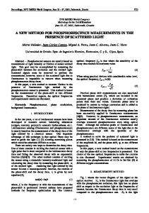
The central issue is ambiguity in the definition of R. For example an approximately rotational component of F may be associated with local advection of enstrophy, rather than generation of enstrophy and hence not correspond to local irreversible mixing (Marshall and Shutts, 1981). The mean dynamics are invariant under any choice of the non-divergent gauge R, but the diffusivity as defined by equation (3) is not. Moreover a diffusivity field diagnosed in this way may be extremely noisy (cf. Nakamura and Chao, 2000), as shown by a sample calculation employing this approach using the simulation data presented in §3. In this diagnostic calculation there are regions of large negative diffusivity, which suggests the presence of strong eddy backscatter (conversion of eddy to mean enstrophy). These negative diffusion regions may be due to pollution of the diagnostic by significant non-divergent eddy PV fluxes and, in this sense, be entirely artificial. Critically, this direct approach fails to unambiguously identify the regions and magnitude of irreversible mixing due to the eddies. Layer 2

Layer 3

κ (m 2 s−1 )

Layer 1

−10000

0

10000

Figure 1: Local eddy PV diffusivities κ (in units of m2 s−1 ), obtained from (3) with R = 0 using the simulation data detailed in §3. Note that the colour scale is saturated.

The gauge freedom may be formally addressed using a horizontal Helmholtz decomposition ˜ ˜ + ˆz × ∇Φ ˜ + H, F = −∇Ψ

(4)

where the first term is the divergent component, the second the rotational component, and the third a harmonic component. Since only the former is directly dynamically active, a down-gradient parameterisation may now alternatively be expressed in terms of the divergent component ˜ = −κΨ˜ ∇q − σΨ˜ ˆz × ∇q, − ∇Ψ

(5)

leading to an alternative definition for the local PV diffusivity κΨ˜ =

˜ · ∇q ∇Ψ |∇q|2 3

.

(6)

Given any divergent component of the eddy PV fluxes one can thus define a local diffusivity (if the mean PV gradient is non-zero) via equation (6). However, in the presence of boundaries, the divergent component is non-unique due to ˜ (Fox-Kemper et al., 2003). Hence the eddy diffusivity freedom in the choice of boundary conditions for the potential Ψ as defined by equation (6) is still not uniquely defined. This ambiguity can be resolved by instead defining a PV diffusivity directly from the eddy PV flux divergence. Specifically, if a pure down-gradient eddy PV flux is postulated, that is, F ≈ −κ∇q,

(7)

then an optimal PV diffusivity can be defined by seeking the spatially varying function κ (x) such that the cost function J (κ) = k∇ · (−κ∇q − F)k2

(8)

is minimised. This defines a best-fit for the diffusivity to the eddy flux divergence. The specific norm, which has been left unspecified for the moment, is a key ingredient in the definition of this optimal diffusivity. Note that a perfect match is not typically to be expected and, moreover, the inversion may be highly ill-conditioned (or even ill-posed). The norm appearing in (8) has an important impact on the structure of the resulting optimal diffusivity. It is clear for example that a simple L2 norm, which leads to Z   2 ∇ · (−κq − F) 2 dΩ, (9) J (κ) = k∇ · (−κq − F)kL2 = Ω

where Ω is the horizontal domain, will lead to difficulties. The divergence of a flux is an inherently noisy quantity, and hence an attempt to optimise the diffusivity to match local structure in the eddy PV flux divergence is likely to be problematic. 2.2. Eddy force function A starting point is to first resolve the non-uniqueness in the definition of the eddy PV flux decomposition in equation (4). This is addressed in Maddison et al. (2015) by noting a relationship between rotational momentum tendencies and divergent eddy PV fluxes, which is briefly summarised. First, it is noted that the QG momentum equation may be written ∂ug = −ˆz × G. ∂t

(10)

Since the geostrophic velocity is non-divergent, ∇ · ug = 0, so −ˆz × G defines a unique rotational momentum tendency. After taking a horizontal curl, G may be identified as a horizontally divergent PV flux. Introducing the stream function ψ such that ug = ˆz × ∇ψ yields ∂ug /∂t = ˆz × ∇Ψ, from which it follows that Ψ=

∂ψ + c(z, t), ∂t

(11)

Following Marshall and Pillar (2011), Ψ is a stream function tendency or force function. In a simply connected domain with no-normal-flow boundary conditions ψ is a (horizontal) constant on all boundaries, and so Ψ inherits a Dirichlet boundary condition. Subject to an appropriate choice of c(z, t) (noting that any other choice vanishes under the horizontal divergence), Ψ satisfies a homogeneous Dirichlet boundary condition. Insisting that the force function decomposition procedure is linear then implies that a force function associated with any single momentum tendency inherits a homogeneous Dirichlet boundary condition. In particular, the eddy force function Ψe is related to the eddy PV flux F = u0 q0 by F = −∇Ψe + ˆz × ∇Φe + He ,

(12)

where Ψe is the solution of a Poisson equation ∇2 Ψe = −∇ · F 4

(13)

subject to homogeneous Dirichlet boundary conditions. The eddy force function has a number of important properties. First, since only the divergence of the eddy PV flux appears in the force function equation (13), it is independent of rotational eddy fluxes. Moreover the eddy force function is inherently smooth. It is shown that, in a simply connected domain, the eddy force function has minimal H01 semi-norm, that is, it is a solution to the Poisson equation (13) for which the mean square gradient is minimised (Maddison et al., 2015, §2 and Appendix A). Note that the eddy force function depends non-locally upon the eddy fluxes — it is related to the flux divergence through an inverse elliptic operator. This suggests that the mis-match function (8) be defined in terms of the mis-match between the eddy force function implied by a parameterisation, and the eddy force function diagnosed from data; that is,

2 J (κ) =

Ψ p (κ) − Ψe

(14) where Ψ p is the parameterised eddy force function computed via ∇2 Ψ p = ∇ · (κ∇q)

(15)

subject to homogeneous Dirichlet boundary conditions. There is now freedom in the definition of the norm appearing in (14). A simple choice is to define this to be the L2 norm, leading to Z h i2

2 Ψ p (κ) − Ψe dΩ. (16) J (κ) = k∇ · (−κ∇q − F)k2 =

Ψ p (κ) − Ψe

L2 = Ω

In technical terms, this is equivalent to defining the norm in the mis-match cost function (8) to be equal to the H0−1 semi-norm. The H0−1 semi-norm places relatively decreased emphasis on high spatial wavenumbers, and hence this definition places relatively increased emphasis on large scale spatial structures in the eddy flux divergence. All results reported in this article use an L2 norm in the definition of the mis-match function, although calculations with other norms (not shown) have been performed and are commented on in the conclusions. 2.3. Constrained optimisation problem for eddy diffusivities Since the force function is defined via the solution of a partial differential equation, it is natural to redefine the optimisation problem considered at the end of §2.1 in terms of a partial differential equation constrained optimisation. For a down-gradient PV parameterisation, letting V ⊆ H01 (Ω) and Vκ ⊆ H 1 (Ω) be real Hilbert spaces, a Lagrange constrained cost function Jˆ : V × V × Vκ → R is defined, where E D

ˆ p , λ, κ) =

Ψ p − Ψe

2 2 + ∇λ, ∇Ψ p − κ∇q + R (κ) . J(Ψ (17) 2 L L

The constrained optimisation problem then seeks a stationary point of the function J(Ψ p , λ, κ). The first term in (17) is the unconstrained function (14), penalising the mis-match between the parameterised and diagnosed eddy force functions. The second term is the weak form partial differential equation constraint. At a ˆ the derivative of Jˆ with respect to λ in any direction φ ∈ V vanishes, leading to stationary point of J, Z D E h i ∇φ, ∇Ψ p − κ∇q 2 = (18) ∇φ · ∇Ψ p − κ∇q dΩ = 0 ∀ψ ∈ V. L

Ω

This is a weak form of the Poisson equation (15), and hence λ is a Lagrange multiplier enforcing the constraint. If the final term is absent, then the solution to the constrained optimation problem finds the optimal κ with minimal force function mis-match. However this problem may be highly ill-conditioned or even ill-posed. The third term can be used to reguarlise the problem by smoothing the resulting diagnosed diffusivity at the expense of optimality. A simple form for this regularisation might, for example, be Z 2 R (κ) =  kκkH 1 =  ∇κ · ∇κ dΩ, (19) Ω

0

where  ∈ R is some parameter chosen to control the smoothness of the resulting optimal κ. 5

ˆ p , λ, κ) all derivatives vanish, yielding the optimality system At a stationary point of the constrained function J(Ψ (e.g., Gunzburger, 2003, §2.2) ∂Jˆ ∂Jˆ ∂Jˆ = 0, = 0, = 0, (20) ∂Ψ p ∂λ ∂κ where formally the derivatives here are Gˆateaux derivatives (e.g., Ch. 17 of Kantorovich and Akilov, 1964). This coupled problem can be solved in its entirety (a “one-shot” approach), and where the problem is non-linear Newton’s method can be applied. For cases where the problem is linear Newton’s method formally converges in one iteration. For the applications considered in this article Newton’s method is applied in all cases, and typically further iterations are applied before tight numerical convergence is reached. This possibly reflects the ill-conditioned nature of the problems considered. A key technical issue encountered here is that the optimality system (20) changes when components of the constrained function are modified; this could arise from a switch of mis-match norm, the form of the parameterisation or the regularisation. If this system is implemented by hand then the code evaluating the left-hand-side needs to be modified for every combination of interest. When Newton’s method is applied, second derivatives are required, exacerbating this issue. To bypass the majority of these problems, the FEniCS automated code generation system is employed (Logg and Wells, 2010; Logg et al., 2012; Alnæs et al., 2014), which enables finite element problems to be described in a high-level syntax and for low-level code to be generated automatically. In the Python front ˆ its Jacobian and compiling and solving of the optimality system (via end, the specification of the cost-function J, code generation and interfacing with external solver libraries) translates to the code outlined in Figure 2. Different schemes can be implemented via small code changes: editing kappa changes the definition of the diffusive closure, J_1 changes the cost function, and J_3 changes the regularisation. Although the code may not be as performant as a hand optimised code, a substantial saving in code development time easily offsets this, and allows a sweep of a large parameter set that would have been otherwise be rather inaccessible. # specify form of kappa kappa = xi ** 2 # form cost function J_1 = ((psi - fns["ffd_empb_%i" % (l + 1)]) ** 2) * dx J_2_res = grad(psi) - kappa * grad(fns["q_%i_n_mean" % (l + 1)]) J_2 = inner(grad(lam), J_2_res) * dx J_3 = eps_marker * (grad(xi) ** 2) * dx J = J_1 + J_2 + J_3 # compute directional derivative dJ = derivative(J, X, du = tests) # solve for the system solve(dJ == 0, X, boundary_conditions, solver_options) Figure 2: Illustrative Python code sample implementing an optimisation problem in FEniCS, for the case of PV diffusion with a positive semidefinite diffusivity, κ = ξ2 . The code specifies the desired variant of the parameterisation, constructs the cost function (“ffd empb %i” and “q %i n mean” are labels for the diagnosed eddy force function associated with the full eddy PV flux and q), and then solves the optimality system.

For all results presented in the article linear systems are solved via SuperLU and SuperLU DIST (Li, 2005; Grigori et al., 2007), via PETSc (e.g., Balay et al., 1997, 2015). 3. Diagnostic calculations for the three-layer simulation In this section the eddy force function and mean fields from an eddy resolving multi-layer QG simulation are used to diagnose eddy diffusivities associated with PV and buoyancy mixing parameterisations. The model is described in Maddison et al. (2015). For completeness, the details of the simulation are presented here.

6

3.1. Simulation details The multi-layer QG equations employed here are (e.g., Pedlosky 1987, §6.16; Vallis 2006, §5.3.2) ∂qi + ∇ · (ug,i qi ) = ν∇2 ωi − rδin ωi + δi1 Qw , ∂t

(21)

where the the layer is counted from top (layer 1) to bottom (layer n), the stream function is defined by ug,i = ˆz × ∇ψi , with ωi = ∇2 ψi . The layer-wise PV qi is related to the stream function ψi via q1 = ∇2 ψ1 + βy + s+1 (ψ2 − ψ1 ), qi = ∇2 ψi + βy + s−i (ψi−1 − ψi ) + s+i (ψi+1 − ψi ), qn = ∇ ψn + βy + 2

where s±i =

s−n (ψn−1

f02 gi±1/2 Hi

=

(22)

− ψn ),

2( f02 /N02 )i±1/2 (Hi + Hi±1 )Hi

(23)

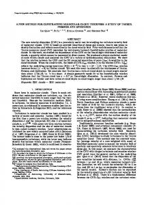
are stratification parameters, Hi is the thickness of layer i, gi+1/2 is the reduced gravity at the interface between layers i and i + 1, N0 is the buoyancy frequency, and f = f0 + βy is the Coriolis parameter. The forcing and dissipation parameters are: a Laplacian viscosity coefficient ν; a bottom friction coefficient r; and the PV tendency due to the wind Qw , with     τ0 2π  yv + D/2      , yv < ym   A sin − π     ρ0 H1 D ym + D/2   (24) Qw =    τ0 2π 1  ym − yv      + ρ H D A sin π D/2 − y  , otherwise, 0 1 m where τ0 is the characteristic magnitude, ρ0 is the reference density, x, y ∈ [0, D], yv = (y − D/2) and ym = B(x − D/2). The zonal and meridional directions are x and y respectively. Zero buoyancy boundary conditions are applied at the top and bottom boundaries (Bretherton, 1966). A partial slip boundary condition ∇2 ψi = −α−1 ∇ψ · nˆ (Haidvogel et al., 1992), where α is a length scale, is applied on the lateral boundaries. A three-layer, double gyre configuration as detailed in Marshall et al. (2012) is used. The equations are discretised in space with a conforming triangle structured mesh with piecewise linear approximation for all fields, a vertex spacing of ∆x = 7.5 km, and implemented using the FEniCS automated code generation system (Logg and Wells, 2010; Logg et al., 2012; Alnæs et al., 2014). The model is discretised in time using a third order Adams–Bashforth scheme with time step size ∆t = 20 mins, using the time-stepping approach detailed in Maddison and Farrell (2014). The equations are integrated for 20,000 days and time averages are taken after this spin-up period for a further 5,000 days. A summary of the relevant parameters is given in Table 1. For further details about the simulation set up, see Marshall et al. (2012) and Appendix B of Maddison et al. (2015); see also Berloff (2005a) and Karabasov et al. (2009) for related configurations of a similar finite difference code on which the finite element code is based. Additional diagnostic quantities were required for the analyis presented here, absent in the simulation data detailed in Maddison et al. (2015), and so the averaging stage was restarted after the 20,000 day spinup. Due to the sensitive dependence on initial conditions and changes in details such as the numerical library versions used, the resulting data are not exactly identical to those presented in Maddison et al. (2015). Eddy force functions for this calculation are shown in Figure 3. 3.2. Eddy diffusivity definition Previously, spatially constant PV diffusivity diagnostics have been reported in Maddison et al. (2015); these generally have limited success in minimising the mis-match between the parameterised and target eddy force function, although this is not unexpected when making a strong assumption of constant diffusivity. Here spatially varying diffusivities are considered. Specifically, we consider a: • general case (GEN), a general signed diffusivity κ(ξ) = ξ(x), supplying no additional information regarding the eddy field and applying no constraints; 7

Layer 2

Layer 3

106 q (s−1 )

Layer 1

0

149 −81

0

81 −81

0

81

0

26 −31

0

31 −62

0

62

2

4

3

1

2

ψ (Sv)

−149

log10 E (ρ0 cm2 s−2 )

−26

0

1.5

0

HΨe (Sv yr−1 )

0

0

1799 −567

0

567 −568

0

568

0

753 −565

0

565 −681

0

681

HΨeb (Sv yr−1 )

−1799

−753

Figure 3: Simulation data for the three-layer finite element ocean gyre calculation over the three layers (columns), with (top to bottom row): final time PV snapshot (in units of s−1 ); time-averaged stream function Hψ (in units of Sv, at 21 contour levels); time-averaged total eddy energy Ei (on a logarithmic scale, in units of ρ0 cm2 s−2 ); eddy force function Hi Ψe,i from the eddy PV flux (in units of Sv yr−1 ); eddy force function Hi Ψeb,i , associated with the buoyancy contribution to the eddy PV flux (in units of Sv yr−1 ). The black contour is the boundary value of the upper layer mean stream function, which approximately indicates the location of the mean jet.

8

parameter D β τ0 ρ0 (A, B) ν r α−1 (H1 , H2 , H3 ) (R1 , R2 ) (s+1 H1 = s−2 H2 , s+2 H2 = s−3 H3 ) ∆x ∆t

value and units 3840 km 2 × 10−11 m−1 s−1 0.08 N m−2 1000 kg m−3 (0.9, 0.2) 100 m2 s−1 4 × 10−8 s−1 120 km (0.25, 0.75, 3.00) km (40, 23) km (2.97, 5.60) × 10−7 m−1 7.5 km 1200 s (= 20 mins)

Table 1: Summary of simulation parameters used for the three-layer finite element ocean gyre calculation, as per Marshall et al. (2012) and Maddison et al. (2015).

• positive semi-definite case (POS), where κ(ξ) = ξ2 (x) ≥ 0 excluding the possibility of negative diffusivity. Note that the corresponding optimality system is inherently non-linear, and that the zero regularisation case is ill-posed (e.g., ξ → −ξ does not change the value of the cost function). Information about the flow may be supplied by, for example, taking κ = f (E)ξ where E is the eddy energy. Diagnostics of this type will be discussed in the conclusions. Considering first diffusion of PV, the layer-wise constrained cost function for PV diffusion takes the form E D

ˆ p,i , λi , ξi ) =

Ψe,i − Ψ p,i

2 2 + ∇λi , ∇Ψ p,i − κ∇qi + R(ξ). (25) J(Ψ 2 L L

The resulting optimisation problem for PV diffusion is vertically decoupled and may be solved layer-wise. The regularisation applied is Z R (ξi ) =  k∇ξi k2H 1 =  ∇ξi · ∇ξi dΩ. (26) Ω

0

For the GEN case this acts to smooth the diffusivity. For the POS case, the regularisation acts on an auxiliary parameter ξi as smoothing the diffusivity directly would result in an optimisation problem of higher order in ξ, leading to additional numerical difficulties. In principle the diagnostic may be computed by seeking a value for the regularisation parameter  which is as small as possible — for example, the value at which the problem becomes sufficiently ill-conditioned for numerical solver failures to be encountered. Instead a desired spatial scale in the parameters is chosen here, seeking a value of the regularisation parameter  to yield a given spatial “roughness”. For this, a non-dimensional roughness measure κr is defined via an appropriately normalised measure of the mean square gradient κ =D r

2

kκk2H 1 0

kκk2L2

R =D

2 Ω

∇κ · ∇κ dΩ R . κ2 dΩ Ω

(27)

An appropriate value of  is found via an iterative procedure as summarised in the pseudo-code in Figure 4. In the majority of cases, this approach yields a final measured roughness that is within 0.5% of a target roughness of κr = 7500; for comparison, a field κ = sin(20πx/D) sin(20πy/D) has κr = 2(20)2 π2 ≈ 7900. In a minority of cases numerical difficulties mean that small values of  cannot be reached (due to numerical solver failures), and in these cases the smallest  at which convergence is achieved is chosen. To quantify the diagnosed diffusivity, six measures are utilised: (i) the mean diffusivity; (ii) an eddy energy weighted mean diffusivity; (iii) a diffusivity positivity measure; (iv) the L2 correlation between the diffusivity and the 9

# initialise parameters theta = 0.5 kappa = kappa_init eps = eps_init while theta < 0.999: # initialise accordingly kappa = solve(..., kappa_init, eps) # decrease epsilon and continue if roughness < tolerance: eps = theta * eps kappa_init = kappa # if tolerance exceeded, try again with larger eps initialised # with previous kappa elif: theta = theta * 4/3 eps = theta * eps Figure 4: Pseudo-code for the procedure employed to select a value of the regularisation parameter  so as to yield a parameter with a given degree of “roughness”. An initial  is chosen and decreased geometrically by some factor θ < 1, until non-convergence or the roughness condition is triggered. The loop is reinitialised at the previously converged solution, with the value of the factor θ increased. This continues until some tolerance for θ is triggered.

eddy energy; (v) the roughness of the diffusivity; (vi) the L2 relative mis-match error between the parameterised and target eddy force function. The mean diffusivity and eddy energy weighted mean diffusivity, are defined via R R κ dΩ Eκ dΩ Ω Ω m R κm = , κ = . (28) E D2 E dΩ Ω Positivity is measured via R κ

>0

=

Ω

H(κ) dΩ

, (29) D2 where H(κ) is the Heaviside function, equal to one where κ ≥ 0 and zero otherwise. The correlation between κ and the eddy energy is measured via R κE dΩ hκ, EiL2 Ω corr (κ, E) = . (30) = qR qR kκkL2 kEkL2 2 dΩ 2 dΩ κ E Ω Ω Note that the correlation is bounded, −1 ≤ corr (κ, E) ≤ 1. The (non-dimensional) roughness of the diffusivity is measured via R kκk2H 1 ∇κ · ∇κ dΩ 0 r 2 2 Ω R κ =D =D . (31) 2 kκkL2 κ2 dΩ Ω Finally mis-match between parameterised and diagnosed force functions is measured via an L2 relative error v u uR  2

t

Ψe − Ψ p

L2 Ψe − Ψ p dΩ Ω R E L2 = = . kΨe kL2 Ψ2 dΩ Ω e

(32)

3.3. Results: PV diffusion Informed by resolution tests, the parameterised force function and parameter ξ are computed on a structured conforming triangle mesh with nodal spacing ∆x = 15 km for all cases presented in the following sections. The diagnosed model force function Ψe,i from the finite element simulation at resolution ∆x = 7.5 km is interpolated 10

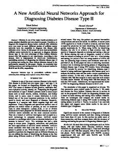
onto this coarser resolution grid via consistent interpolation (evaluation of the higher resolution data at the vertices of the coarse grid). Figure 5 shows the diffusivity κ diagnosed for the GEN and POS diffusivity variants. The local mis-match is shown in Figure 6. Values for the diagnostic quantities from equation (28) to (32) are summarised in Figure 7. Layer 2

Layer 3

POS

GEN

Layer 1

−10000

0

10000

Figure 5: The diffusivity κ (in units of m2 s−1 ) associated with PV diffusion over the three layers (columns), for the GEN case κ = ξ (top row) and POS case κ = ξ2 ≥ 0 (bottom row). The colour scale is fixed and saturated.

Starting with the GEN case, there are regions of negative diffusivity towards the eastern boundary in the upper and middle layers, and a correspondingly large positive diffusivity towards the western boundary, at least in the upper layer. This is consistent with the signal that might be associated with a westward propagating of eddy activity. There is a second pool of negative diffusivity towards the down-stream mean jet in the upper layer. This is consistent with an outward flux of activity due to the “wave radiator” mechanism discussed in Waterman and Jayne (2011, 2012) for the stable down-stream region of an inertial barotropic jet. In the middle layer, a comparison with the mean streamlines ψ in Figure 3 (second row) reveals that the closed streamlines north and south of the jet correlate with regions of positive diffusivity. This is in agreement with the principle of PV homogenisation within closed streamlines (Rhines and Young, 1982). A similar correlation exists in the upper layer, though this is less strong; this correlation breaks down to the north of the mean jet, possibly due to the presence of strong wind forcing in this layer. There are signals of negative diffusivity in the upper layer confined close to the northern and southern boundaries. This signal can be expected if there is a local eddy activity backscatter owing to the presence of Fofonoff gyres in these regions (e.g., Berloff, 2005b; Marshall and Adcroft, 2010). In the lower layer, the diffusivity is large and positive in the jet, correlating with the location of the largest eddy energy. However in this layer there are meridionally oriented patterns in the diffusivity away from the jet. This “banding” correlates with a similar pattern in the local mis-match in Figure 6, and so it is possible that this signal is a numerical artefact. A similar effect may account for the alternating diffusivity sign in the upper layer mean jet. It is apparent that there are regions of significant negative diffusivity. For the GEN case, in the middle layer unweighted and eddy energy weighted means are positive and of a similar magnitude (around 750 and 1200 m2 s−1 respectively), indicating that the diffusivity is largely positive in this layer. This is supported by the positivity index in the middle layer at around 60%. Some degree of correlation between eddy energy and diffusivity is seen. The roughness is found to be well controlled by the solution output criterion; it has 11

Layer 2

Layer 3

POS

GEN

Layer 1

−1

0

1





Figure 6: Layer-wise non-dimensional mis-match D Ψe,i − Ψ p,i /

Ψe,i

L2 associated with PV diffusion over the three layers (columns), for the GEN case κ = ξ (top row) and POS case κ = ξ2 ≥ 0 (bottom row). The colour scale is fixed and saturated in layer 1.

3000

(a) κm E

1000

0 GEN

GEN 10000

(d)

0

POS

50

(e)

GEN

POS Layer 1 Layer 2 Layer 3

(f)

EL2

40 κr

corr(κ, E)

POS

0.4

5000

0.2 0

50

1000

0

0.6

(c)

2000

κm

2000

100

(b) κ>0

3000

30 20 10

GEN

POS

0

GEN

POS

0

GEN

POS

Figure 7: Bar graphs comparing the diagnostic data across the three layers of for the GEN and POS associated with PV diffusion : (a, b) the mean >0 from equation (29); (d) the correlation corr(κ, E) from κm and the eddy energy weighted mean κm E from equation (28); (c) the positivity index κ equation (30); (e) the roughness κr from equation (31); ( f ) the relative L2 error EL2 from equation (32).

12

been confirmed that the κ output is within 0.5% of the fixed target roughness. Given this, we see that the resulting L2 relative error is low, at less than 2%. In the lower layer the eddy energy weighted mean is smaller, and the unweighted mean in negative. While the error in the inversion is well controlled, at less than 1%, the banding of positive and negative diffusivities away from the jet in this case lead to a negative unweighted mean. This may reflect difficulties in the diagnostic in this region. In the upper layer the diffusivity, while positive in the means, exhibits almost no correlation with the eddy energy and, for a given roughness, the relative L2 mis-match is greater than in the other two layers. The POS case shows similar patterns of positive diffusivity around the location of the mean jet and towards the western boundary. However, this diagnostic shows large regions of very low diffusivity, which typically correlate with regions of negative diffusivity seen in the GEN case. In the middle and lower layer the correlation between diffusivity and eddy energy has increased compared to the GEN case. The corresponding relative L2 mis-match is slightly larger than the GEN case, by at less than 5% for a similar level of roughness. In the upper layer the L2 mismatch is much larger, at around 30%, and a very low correlation between diffusivity and eddy energy is observed. On closer inspection of the spatial distribution of error, seen in Figure 6, the errors are generally large around the mean jet. This is particularly the case in the upper layer. In summary, the diagnostic calculations produce a diffusivity field that correlates with some physical processes that are known to occur. In the middle and lower layer, both diffusivity variants shows a strong positive signal that has some correlation with the eddy energy and, for a given roughness, the resulting L2 mis-match is low. The same cannot be said for the diganosed diffusivity in the upper layer, where the correlation between eddy energy and diffusivity is low, and the errors are significantly larger for a given roughness. It appears that a negative signal is a prevalent especially in the upper layer; for a given roughness, the POS case has associated with it significantly larger mis-match error. 3.4. Results: Buoyancy mixing An analogous procedure may be applied to the down-gradient mixing of buoyancy u0 b0 = −κgm ∇b,

(33)

which, in the QG setting, is equivalent to the Gent–McWilliams (GM) parameterisation (Gent and McWilliams 1990; see also Treguier et al. 1997). The analogous constrained cost function in the continuously stratified setting is given by   +  *   Z 0 

2



2   ∂  f0  ˆ J Ψ p , λ, κgm = (34)  κgm ∇b +  ∇κgm L2  dz,  Ψeb − Ψ p L2 + ∇λ, ∇Ψ p − ∂z N02 z=−H L2 where all inner products and norms are defined via integration over the horizontal domain. The eddy force function associated with the buoyancy fluxes is shown in the lower row of Figure 3. In the multi-layer quasi-geostrophic equations the buoyancy flux and ∇b are defined on interfaces and so, via equation (33), κgm is also interfacial. The corresponding PV flux is related to the interfacial buoyancy flux via a vertical derivative operator (Greatbatch and Lamb, 1990). This introduces vertical coupling, and as such the corresponding optimisation problem for κgm is fully three-dimensional, unlike the previous PV diffusion case. An alternative method, not pursued here, is to define an interfacial eddy stress function (Maddison et al., 2015, Appendix C), and use this as the basis for an κgm diagnostic computed separately on each interface. The eddy buoyancy fluxes on each interface (R, S ) = ( f02 /N02 )u0 (∂ψ0 /∂z) may be defined ! ! 1 ∂ 1 ∂ + Ri+1/2 = − S i+1/2 = + (35) (ψi + ψi+1 ) Hi si (ψi − ψi+1 ), (ψi + ψi+1 ) Hi s+i (ψi − ψi+1 ), 2 ∂y 2 ∂x with stratification parameters s+i as given by (23). Vertical differencing then leads to a discrete eddy PV flux associated with the eddy buoyancy fluxes (i.e. these are the vertical stresses appearing in a vertically discrete Taylor–Bretherton identity (Maddison et al., 2015, appendix B). The interfacial GM coefficient is then defined via   
Ri+1/2 , S i+1/2 = Hi s+i −(κgm )i+1/2 ∇ ψi − ψi+1 . (36) 13

Again, the GEN case κgm = ξ and POS case κgm = ξ2 are considered. The vertically discrete cost function for the buoyancy mixing case is given by Jˆ =

3 2 D X X E

2  Hi + Hi+1

H (Ψ − Ψ )

2 + +

∇ξ − ψ ) +  ∇λ , ∇Ψ + H s (κ ) (ψ i+1/2 L2 . i eb,i p,i L2 i p,i i i gm i+1/2 i i+1 L2 2 i=1 i=1

(37)

The regularisation again penalises gradients in κgm , but without increasing the order for the resulting optimisation problem for the POS case. The procedure for implementation, solving the variational problem, simulation details, manner of decreasing  and output of solution based on the roughness criteria (with target roughness of 7500 as for the PV diffusion case) are as detailed in the previous subsection, where the roughness is now defined to be  2  X

2   Hi + Hi+1



∇κgm, i+1/2

L2  2 i=1 r (38) κgm = D2 . 2  X

2   Hi + Hi+1

 

κgm, i+1/2 L2  2 i=1 The resulting interfacial GM coefficients are shown in Figure 8, and the local mis-matches are shown in Figure 9. The same diagnostic quantities from equation (28) to (32) are employed to assess the resulting diffusivity, and these are summarised in Figure 10. Interface 1

Interface 2

−10000

(b)

Interface 1

POS

GEN

(a)

0

10000

Figure 8: The diffusivity κgm (with units of m2 s−1 ) on the interfaces associated with buoyancy mixing. (a) the GEN case κgm = ξ for both interfaces; (b) the POS case with κgm = ξ2 for upper interface only, as the lower interface is the zero solution. The colour scale is fixed and saturated.

Consider first the GEN case, shown in Figure 8(a). In the upper interface κgm is positive in the north-west and south-west corners. A large region of positive κgm exists in the southern gyre. There is a significant pattern of negative κgm , particularly to the north of the mean jet and in the downstream mean jet. In the lower interface, κgm is predominantly negative around the down-stream mean jet. This negative coefficient is consistent with previously reported signals of baroclinic stability here, described in Berloff (2005a) and Maddison et al. (2015). Away from the jet there is a positive κgm region towards the north-east, but negative κgm in the southern gyre. The unweighted and the eddy energy weighted means are negative, especially in the lower interface. The positivity index is low, below 50%, and the correlation between κgm and the eddy energy is low and negative, indicating the prevalence of a negative signal and a weak correlation with eddy energy. The L2 relative errors however are reasonable, at less than 10% for both interfaces. An observation to be made here is that, unlike the PV diffusion case, here the upper layer has the lowest mis-match. That is, the use of a global mis-match cost function here has led to a preferential decrease in the upper layer mis-match, at the expense of the lower two layers. Now considering the POS case, the lower layer diffusivity is zero (not shown). This was found to be robust even after, in the algorithm of Figure 4, choosing multiple initial values of  and multiple initial guesses for the ξ field. 14

Layer 2

Layer 3

POS

GEN

Layer 1

−1

0

1

 

Figure 9: Layer-wise non-dimensional mis-match D Ψeb,i − Ψ p,i /

Ψeb,i

L2 associated with buoyancy mixing over the three layers (columns), for the GEN case κgm = ξ (top row) and the POS case κgm = ξ2 ≥ 0 (bottom row). The colour scales are fixed and saturated in the upper and bottom layer for the GEN case and across all layers in the POS case.

1500

(a)

(c)

1000 κm E

κm

1000

100

(b)

500

κ>0

1500

500

0

50

0

−500

GEN

POS

−500

GEN

0

POS

GEN

POS

4

2

(d)

100

(e)

Interface 1 Interface 2

1.5

0 −0.1 −0.2

x 10

EL2

0.1 κr

corr(κ, E)

0.2

1

Layer 1 Layer 2 Layer 3

(f)

50

0.5 GEN

POS

0

GEN

POS

0

GEN

POS

Figure 10: Bar graph comparing the diagnostic data across the two interfaces and three layers of the GEN and POS case for buoyancy mixing: (a, b) >0 and eddy energy weighted positivity index the mean κm and the eddy energy weighted mean κm E from equation (28); (c, d) the positivity index κ >0 r 2 κE from equation (29); (e) the roughness κ from equation (31); ( f ) the relative L error EL2 from equation (32). Note that the lower interface solution for the POS case is zero.

15

The existence of a global minimum with non-zero lower interface κgm cannot be ruled out. In the upper interface, however, a non-zero solution is found, with a strong positive signal in the southern gyre and towards the northwestern and south-western boundaries. Here, regions of low diffusivity correlate well with the regions of negative diffusivity previously observed in the GEN case. The associated error is large almost everywhere, as seen in Figure 9 and Figure 10( f ). In summary, the GEN case diagnosed diffusivity shows strong negative signals, for example in the lower interface down-stream mean jet. Enforcing positive semi-definite diffusivity in the POS case leads to very significantly increased mis-match errors, and difficulty in diagnosing a non-trivial diffusivity in the lower interface. The correlation with eddy energy is, in both cases, low. A key issue encountered here is that, in a three-layer configuration, each of the two interfaces is coupled to layers which experience either direct wind forcing or bottom dissipation. Hence more significant influence from forcing and dissipation may be expected in these diagnostics. This is addressed in the following section by adding an increased number of model layers. 4. Results: Five layers, potential vorticity and buoyancy mixing A five layer simulation is performed using a higher horizontal resolution model with a grid spacing of ∆x = 3.25 km, using a finite difference code (see e.g., Berloff (2005a), and particularly Karabasov et al. (2009) for the CABARET numerical scheme which is used here). Parameter values that differ from the earlier three-layer calculation are given in Table 2. Stratification parameters are based upon stratification profiles from the World Ocean Circulation Experiment (Gouretski and Kolterman, 2004; Koltermann et al., 2011) data, employing a density profile of the form ρ(z) = a + bez/c (noting that z = 0 is the top of the ocean); specific values of a, b and c as well as f0 are also given in Table 2. Note that the leading baroclinic deformation radii are somewhat lower than the earlier three-layer calculation. parameter ν (H1 , H2 , H3 , H4 , H5 ) (R1 , R2 , R3 , R4 ) s+1 H1 = s−2 H2 s+2 H2 = s−3 H3 s+3 H3 = s−4 H4 s+4 H4 = s−5 H5 ∆x ∆t a b c f0

value and units 10 m2 s−1 (0.15, 0.29, 0.58, 1.16, 2.32) km (33, 17, 11, 10) km 8.09 × 10−7 m−1 7.24 × 10−7 m−1 1.16 × 10−6 m−1 5.90 × 10−6 m−1 3.25 km variable, based on the Courant number 1000 kg m−3 1.2 kg m−3 500 m  ◦   50 π 2π  s−1 sin  3600 × 24 180◦ 

Table 2: Simulation parameters used for the five-layer finite difference ocean gyre calculation. Other parameters employed are as per Table 1.

Diagnostic calculations are repeated for this case via interpolation of the finite difference data onto the earlier finite element mesh with a nodal spacing of ∆x = 15 km. Diffusivities are then diagnosed as before. 4.1. Potential vorticity diffusion The corresponding eddy force function Ψe and total eddy energy distribution E for the five-layer calculation are largely similar in structure to the three layer case shown in Figure 3. As a consequence of this the resulting PV diffusivities associated with the GEN and POS cases, displayed in Figure 11, show largely similar structures to the three-layer case. The associated diagnostic quantities from equation (28) to (32) are summarised in Figure 12. Considering first the GEN case, the resulting diffusivity is predominantly positive over all layers, though still possessing significant local negative signals particularly in the upper layer. The rapidly varying structure within the 16

Layer 2

Layer 3

Layer 4

Layer 5

ψ (Sv)

Layer 1

0

13 −17

0

17 −19

0

19 −28

0

28 −53

0

53

POS

GEN

−13

−10000

0

10000

Figure 11: Contours of ψ (with units of Sv) at 21 contour levels (top row) and the diffusivity κ (with units of m2 s−1 ) associated with the GEN case κ = ξ (middle row) and POS case κ = ξ2 ≥ 0 (bottom row) for PV diffusion over the five layers (columns). The colour scale for the diffusivity is saturated.

6000

(a) κm E

2000

0

POS

10000

(d)

GEN

0

POS

50

(e)

GEN

POS Layer 1 Layer 2 Layer 3 Layer 4 Layer 5

(f)

40

0.4

EL2

κr

corr(κ, E)

GEN

0.6 5000

0.2 0

50

2000

0

0.8

(c)

4000

κm

4000

100

(b) κ>0

6000

30 20 10

GEN

POS

0

GEN

POS

0

GEN

POS

Figure 12: Bar graph comparing the diagnostic data across the five layers of the GEN and POS case associated with down-gradient PV diffusion: >0 and eddy energy weighted positivity (a, b) the mean κm and the eddy energy weighted mean κm E from equation (28); (c, d) the positivity index κ >0 r 2 index κE from equation (29); (e) the roughness κ from equation (31); ( f ) the relative L error EL2 from equation (32). The lowest layer for the POS case has not been returned via triggering the roughness criterion, and instead the last converged solution has been returned.

17

mean jet is present but may again be seen to be correlated with the locations of largest local error (not shown; cf. Figure 6). In layer three there are suggestions of a boundary confined negative signal near the north and southern boundaries. There is also a suggestion of a negative signal around the mean jet in the second and third layers. There is again correlation between locations of positive diffusivity within contours of closed stream lines ψ, especially in the third and fourth layers. The overall positivity for the diagnosed diffusivity is generally high (see Figure 12a, b, c). Further, there is mild correlation between the diffusivity and the eddy energy and, for the same given roughness as in the three layer case, the resulting L2 mis-match errors are all less than 10%. The mis-match is particularly low away from the upper layer. For the POS case, the observations are again similar to those made for the three layer case. The regions of positive diffusivity in the GEN and POS case largely coincide, with strong positive diffusivity in the southern gyre and western boundary. These regions of positive diffusivity again correlate well with the locations where there are closed mean stream lines. Regions of low diffusivity also correlate well with the regions of negative diffusivity present in the GEN case. There is again evidence of correlation between the diffusivity and the eddy energy especially in the lower layers and, for a given roughness, the L2 mis-match is reasonable away from the upper layer. It should be noted that the bottom layer solution for the POS case has not converged to the target roughness, though the errors are still less than 10%. 4.2. Buoyancy mixing In the five-layer configuration there are two interfaces which are free from the direct influence of upper layer forcing and bottom drag. These internal interfaces are therefore likely to show a signal more consistent with the quasi-adiabatic ocean interior, and hence more likely to correlate with the action of down-gradient buoyancy mixing. The resulting κgm for the GEN and POS case are shown in shown in Figure 13. The relevant diagnostic quantities are summarised in Figure 14. Interface 2

Interface 3

Interface 4

POS

GEN

Interface 1

−10000

0

10000

Figure 13: The diffusivity κgm (with units of m2 s−1 ) associated with the GEN case κgm = ξ (top layer) and POS case κgm = ξ2 (bottom layer) for buoyancy mixing over the four interfaces (column). The colour scale is saturated to show the spatial structures. Note that the GEN solution has not r converged at the target global roughness of 7500 (see equation 38), but instead the last converged solution at κgm ≈ 1100 is displayed here.

18

3000

3000

2000

2000

1000

100

(b) κ>0

4000

(a) κm E

κm

4000

Interface 1 Interface 2 Interface 3 Interface 4

(c)

50

1000

0

0 GEN

POS

GEN

0

POS

GEN

POS Layer 1 Layer 2 Layer 3 Layer 4 Layer 5

4

(d)

x 10

50

(e) EL2

0.2

1 0.5

0 GEN

POS

0

(f)

40

1.5 κr

corr(κ, E)

0.4

2

30 20 10

GEN

POS

0

GEN

POS

Figure 14: Bar graph comparing the diagnostic data across the four interfaces and five layers for the GEN and POS case associated with buoyancy >0 and eddy mixing parameterisations: (a, b) the mean κm and the eddy energy weighted mean κm E from equation (28); (c, d) the positivity index κ >0 r 2 energy weighted positivity index κE from equation (29); (e) the roughness κ from equation (31); ( f ) the relative L error EL2 from equation (32). r Note here is that the GEN case did not converge around the target global roughness of κgm = 7500 (see equation 38); instead, the last converged r solution at κgm ≈ 1100 is displayed here.

r The first thing to note here is that the GEN case did not converge around the target global roughness of κgm = 7500; r instead, the last converged solution at κgm ≈ 1100 is displayed here. This fact is perhaps noticeable in that the diagnosed diffusivity is rather smooth, certainly compared to the three-layer case displayed in Figure 8(a). However, the physical features are still robust, with the presence of the negative signal down-stream of the mean jet across all interfaces, and the positive diffusivity in the southern gyre, the western boundary and in the north-west region. The mean is now largely positive except in the lowest interface, where it is mildly negative. The eddy energy weighted mean however is mostly negative and small in magnitude. The positivity index shows the diffusivity generally takes positive values over the domain, although clear negative signals around the mean jet are observed. The correlation between the diffusivity and the eddy energy is generally small and negative. The roughness varies over the interfaces r because of the layer weighting employed in the definition of the global roughness κgm . Given the resulting calculation 2 possesses a rather low roughness, the relative L mis-match is respectable, at less than 20% over all fiver layers. The upper layer again has the lowest mis-match. For the POS case a non-zero solution is now found over all interfaces, in marked contrast the earlier three layer case. The locations of positive signals again correlate well with the locations of the positive signals observed in the GEN case. The locations of low diffusivity in the POS case also correlate well with the locations of negative signals in the GEN case. The unweighed mean and especially the eddy energy weighted mean are by construction positive — the latter has a value of order 1300 m2 s−1 . The correlation between the diffusivity and the eddy energy is larger than in the GEN case. However, given that the POS case has a higher parameter roughness (noting the less rough GEN case solution), the associated mis-match is still significantly larger. This suggests that negative κgm is required for an accurate match between the target and the parameterised eddy force functions.

5. Conclusions A new method for diagnosing eddy diffusivities in a gauge-invariant fashion, independent of dynamically inactive rotational flux components, has been presented. This is achieved by seeking to match diagnosed and parameterised eddy force functions through a one-shot optimisation procedure. The eddy force function depends only upon eddy flux divergences, through an inverse elliptic operator, and hence the force function is inherently smooth and non-local.

19

The optimisation problem allows control over the roughness of the resulting diffusivity field. Combined, this method yields an optimal diffusivity that is gauge-invariant, non-local and has controlled smoothness. The approach has been applied to multi-layer quasi-geostrophic ocean gyre simulations. Results have been shown here for data obtained from a three-layer finite element simulation and a five-layer higher resolution finite difference simulation. The diagnostic method has been applied for down-gradient PV mixing and buoyancy mixing with a general unconstrained diffusivity and a positive semi-definite diffusivity. The resulting optimality systems were implemented using the FEniCS automated code generation system. Here the code generator greatly facilitates parameterisation testing, as new methods can be implemented and tested via small code modifications, and these changes are propagated automatically. In particular, cost function Jacobians and Hessians are formulated automatically via high-level algorithmic differentiation, and specific code for the assembly of these discrete operators is generated automatically. Regarding down-gradient PV mixing parameterisations, the key conclusions are that: (i) there are robust locally negative diffusivities that are present even in the absence of rotational fluxes, although the mean diffusivity over the horizontal domain is positive; (ii) the optimisation has success in matching the eddy force function diagnosed from an eddying calculation in the lower layers, but has less success in the upper layer where there is strong wind forcing present; (iii) the locations of closed mean recirculations often correlate with signals of positive diffusivity; (iv) there is positive correlation between the eddy energy and the diffusivity in the lower layers. For down-gradient buoyancy mixing, negative signals are again present, although in this instance some of this is attributed to the lack of vertical resolution in the three-layer calculation. The five-layer calculations indicate predominantly positive eddy diffusivities away from the location of the mean jet, albeit with some strong negative signals in the southern part of the lower two interfaces. Notwithstanding this exception, this is consistent with the action of down-gradient momentum transfer input by the wind through the action of baroclinic instability. However, within the mean jet, and particularly in the lower layer and down-stream jet regions, the eddy diffusivity is strongly negative, suggesting local baroclinic stability, and forcing of the mean jet baroclinicity by the eddy buoyancy fluxes. These results are consistent with the earlier observations reported in Berloff (2005a) and Maddison et al. (2015). Throughout this paper the mis-match measure was defined via an L2 norm, measuring the mis-match between the diagnosed and parameterised eddy force functions. Additional calculations were performed using a H01 mis-match measure, which measures the mis-match between diagnosed and parameterised divergent eddy fluxes. The solutions obtained from the H01 based mis-match norms result in higher relative L2 mis-matches; this may be attributed to the fact that the H01 case places more emphasis on the local, small-scale features over the global, large-scale features. Calculations which attempted to directly match diagnosed and parameterised eddy flux divergences (respectively, ∇2 Ψe and ∇ · (−κ∇q)) were not successful. It is possible to consider diagnostics which seek diffusivities which are themselves defined in terms √ of the eddy energy (e.g., ?Eden and Greatbatch, 2008). For example, one could consider the definition κ = Eξ, where ξ a mixing length, or alternatively κ = Eξ, where here ξ is a time-scale. Via either of these approaches a given roughness in the underlying parameter ξ permits an increased roughness in κ; that is, the eddy energy may be used to provide additional information on the spatial structure of the diffusivity. Such diagnostics have been investigated (not shown) and yield a root-mean-square mixing length of 15–40 km, and a root-mean-square time scale of 3–10 days. The latter time-scale is similar to that described in McWilliams and Gent (1994) for an eddy kinetic energy dependent variant of GM with a spatially varying coefficient. For the purposes of eddy parameterisation, the diagnosed PV diffusivities exhibit some desirable features. The mean diffusivity (either unweighted or eddy energy weighted) is positive, and is generally also locally positive (notwithstanding some regions of strong negative diffusivity, particularly in the upper layer). The positive correlation of the diffusivity with eddy energy, while somewhat modest, provides some additional support to the principle of eddy energy based eddy parameterisations, for example as discussed in, Eden and Greatbatch (2008), Cessi (2008), Marshall and Adcroft (2010) and Jansen and Held (2013). Enforcing a positive semi-definite diffusivity leads to an increased error at the selected parameter roughness. Indeed this latter approach generally leads to a similar spatial diffusivity pattern as obtained with an unconstrained diffusivity, but with negative diffusivities deleted, and somewhat larger positive diffusivities elsewhere. Diagnosed interfacial buoyancy diffusivities are, for the purposes of eddy parameterisation, potentially more problematic. In particular, at least in the five layer calculation, where the influence of forcing and dissipation is weaker for the intermediate layers, there are large scale and large magnitude negative diffusivity signals, particularly 20

in the region of the mean jet. While there are also strong postive signals away the jet, the eddy energy weighted mean and the correlation with the eddy energy are both negative. Enforcing a positive semi-definite diffusivity again generally leads to a similar pattern of positive spatial diffusivies, with larger magnitude, and with negative signals deleted. The mis-match in this latter case, at the selected roughness, is also significantly increased. There do appear to be some robust structures appearing in the diagnosed potential vorticity diffusivities. The five layer calculations suggest signals broadly consistent with down-gradient diffusivities, hinting that such a closure may be tractable here. This observation comes with the caveat that, in general, a down-gradient potential vorticity closure violates momentum conservation (e.g., Marshall, 1981; Marshall et al., 2012) through the failure to preserve the underlying tensorial structure resulting from the Taylor-Bretherton identity (e.g., Griffies, 2004; Popovych and Bihlo, 2012; Maddison and Marshall, 2013). The diagnosed buoyancy diffusivities imply a region near the mean jet with a robust negative diffusivity imply a region with robust negative diffusivity, consistent with the action of baroclinic stability. This suggests that, at least in the regions of strong lateral shear, a closure for eddy buoyancy fluxes should permit a degree of backscatter. This is not typically captured within current eddy parameterisation schemes. The optimisation procedure may potentially be extended to the primitive equations, provided an analogous eddy force function may be defined. One could consider, for example, a force function defined as in Marshall and Pillar (2011). A practical limitation here is likely to be the difficulty of solving the associated ill-conditioned optimality systems. In this article this was addressed by reducing the size of the problems, through interpolation onto a coarser mesh, combined with the use of direct solvers which are practical for these problem sizes. For larger problems more advanced methods, such as the use of iterative methods with appropriate pre-conditioners for the relevant linear systems, are likely to be required. In practice a parameterisation quality may not necessarily be determined by its ability to represent eddy statistics themselves. That is, it may be acceptable for a given parameterisation to imply a differing eddy diffusivity if it nevertheless yields a high quality mean state. A more advanced method of diagnosing eddy diffusivities, for example, could seek to invert for a diffusivity which yields an optimal mis-match between high resolution and parameterised mean states. Such a diagnostic would apply the dynamical equations themselves as a constraint on the optimisation, and replace the unconstrained cost function used here with a mis-match measure defined in terms of the deviation of the parameterised model from the target high resolution reference. Acknowledgements This work was funded by the UK Natural Environment Research Council grant NE/L005166/1. This work used the ARCHER UK National Supercomputing Service (http://www.archer.ac.uk). The parallel finite difference code used in this article is based upon an earlier code provided by P. S. Berloff (see also Karabasov et al., 2009). The data used for generating the plots in this article is available through the Edinburgh DataShare service at http://dx.doi.org/10.7488/ds/366. References Alnæs, M. S., Logg, A., Ølgaard, K. B., Rognes, M. E., Wells, G. N., 2014. Unified Form Language: A domain-specific language for weak formulations of partial differential equations. ACM Trans. Math. Softw. 40, 9:1–9:37. Balay, S., Abhyankar, S., Adams, M. F., Brown, J., Brune, P., Buschelman, K., Dalcin, L., Eijkhout, V., Gropp, W. D., Kaushik, D., Knepley, M. G., Curfman McInnes, L., Rupp, K., Smith, B. F., Zampini, S., Zhang, H., 2015. PETSc users manual. Tech. Rep. ANL-95/11 - Revision 3.6, Argonne National Laboratory. URL http://www.mcs.anl.gov/petsc Balay, S., Gropp, W. D., McInnes, L. C., Smith, B. F., 1997. Efficient management of parallelism in object-oriented numerical software libraries. In: Arge, E., Bruaset, A. M., Langtangen, H. P. (Eds.), Modern Software Tools in Scientific Computing. Birkh¨auser Boston, pp. 163–202. Berloff, P., 2005a. On dynamically consistent eddy fluxes. Dyn. Atmos. Ocean. 38, 123–146. Berloff, P., 2005b. On rectification of randomly forced flows. J. Mar. Res. 63, 497–527. Bretherton, F. P., 1966. Critical layer instability in baroclinic flows. Q. J. Roy. Met. Soc. 92, 325–334. Cessi, P., 2008. An energy-constrained parametrization of eddy buoyancy flux. J. Phys. Oceanogr. 38, 18071819. Eden, C., Greatbatch, R. J., 2008. Towards a mesoscale eddy closure. Ocean Modell. 20, 223–239. Eden, C., Greatbatch, R. J., Olbers, D., 2007. Interpreting eddy fluxes. J. Phys. Oceanogr. 37, 1282–1296. Fox-Kemper, B., Ferrari, R., Pedlosky, J., 2003. On the indeterminacy of rotational and divergent eddy fluxes. J. Phys. Oceanogr. 33, 478483. Gent, P. R., McWilliams, J. C., 1990. Isopycnal mixing in ocean circulation models. J. Phys. Oceanogr. 20, 150–155.

21

Gouretski, V. V., Kolterman, K. P., 2004. WOCE global hydrographic climatology. Ber. Bundesamte Seeschifffahrt Hydrogr. Rep. 35. Greatbatch, R. J., Lamb, K. G., 1990. On parametrizing vertical mixing of momentum in non-eddy resolving ocean models. J. Phys. Oceanogr. 20, 1634–1637. Green, J. S. A., 1970. Transfer properties of the large-scale eddies and the general circulation of the atmosphere. Q. J. Roy. Met. Soc. 96, 157185. Griesel, A., Gille, S. T., Sprintall, J., McClean, J. L., Maltrud, M. E., 2009. Assessing eddy heat flux and its parameterization: A wavenumber perspective from a 1/10◦ ocean simulation. Ocean Modell. 29, 248–260. Griffies, S. M., 2004. Fundamentals of Ocean Climate Models. Princeton University Press. Grigori, L., Demmel, J. W., Li, X. S., 2007. Parallel symbolic factorization for sparse LU with static pivoting. SIAM J. Sci. Comput. 29, 1289–1314. Gunzburger, M. D., 2003. Perspectives in flow control and optimization. Advances in design and control. SIAM. Haidvogel, D. B., McWilliams, J. C., Gent, P. R., 1992. Boundary current separation in a quasigeostrophic, eddy-resolving ocean circulation model. J. Phys. Oceanogr. 22, 882–902. Jansen, M. F., Held, I. M., 2013. Parameterizing subgrid-scale eddy effects using energetically consistent backscatter. Ocean Modell. 80, 36–48. Jayne, S. R., Marotzke, J., 2002. The oceanic eddy heat transport. J. Phys. Oceanogr. 32, 3328–3345. Kantorovich, L. V., Akilov, G. P., 1964. Functional analysis in normed spaces. Vol. 46 of International series of monographs in pure and applied mathematics. Pergamon Press, translator D. E. Brown. Karabasov, S. A., Berloff, P. S., Goloviznin, V. M., 2009. CABARET in the ocean gyres. Ocean Modell. 30, 155168. Koltermann, K. P., Gouretski, V. V., Jancke, K., 2011. Hydrographic Atlas of the World Ocean Circulation Experiment (WOCE). Volume 3: Atlantic Ocean. M. Sparrow, P. Chapman and J. Gould (Eds.), International WOCE Project Office, Southampton, UK, ISBN 090417557X. Li, X. S., 2005. An overview of SuperLU: Algorithms, implementation, and user interface. ACM Trans. Math. Softw. 31, 302–325. Logg, A., Mardal, K. A., Wells, G. N., 2012. Automated Solution of Differential Equations by the Finite Element Method. Springer. Logg, A., Wells, G. N., 2010. DOLFIN: Automated finite element computing. ACM Trans. Math. Softw. 37, 20:1–20:28. Maddison, J. R., Farrell, P. E., 2014. Rapid development and adjoining of transient finite element models. Comput. Methods Appl. Mech. Engrg. 276, 95–121. Maddison, J. R., Marshall, D. P., 2013. The Eliassen–Palm flux tensor. J. Fluid Mech. 729, 69–102. Maddison, J. R., Marshall, D. P., Shipton, J., 2015. On the dynamical influence of ocean eddy potential vorticity fluxes. Ocean Modell. 92, 169–182. Marshall, D. P., Adcroft, A. J., 2010. Parameterization of ocean eddies: Potential vorticity mixing, energetics and Arnolds first stability theorem. Ocean Modell. 32, 1571–1578. Marshall, D. P., Maddison, J. R., Berloff, P. S., 2012. A framework for parameterizing eddy potential vorticity fluxes. J. Phys. Oceanogr. 42, 539–557. Marshall, D. P., Pillar, H. R., 2011. Momentum balance of the wind-driven and meridional overturning circulation. J. Phys. Oceanogr. 41, 960–978. Marshall, J. C., 1981. On the parameterization of geostrophic eddies in the ocean. J. Phys. Oceanogr. 11, 257–271. Marshall, J. C., Shutts, G. J., 1981. A note on rotational and divergent eddy fluxes. J. Phys. Oceanogr. 11, 1677–1680. McDougall, T. J., McIntosh, P. C., 1996. The temporal-residual-mean velocity. Part I: Derivation and the scalar conservation equations. J. Phys. Oceanogr. 26, 2653–2665. McWilliams, J. C., Gent, P. R., 1994. The wind-driven ocean circulation with an isopycnal-thickness mixing parameterization. J. Phys. Oceanogr. 24, 46–65. Medvedev, A. S., Greatbatch, R. J., 2004. On advection and diffusion in the mesosphere and lower thermosphere: The role of rotational fluxes. J. Geophys. Res. 109 (D07104). Nakamura, M., 1998. On modified rotational and divergent eddy fluxes and their application to blocking diagnoses. Q. J. Roy. Met. Soc. 124, 341–352. Nakamura, M., Chao, Y., 2000. On the eddy isopycnal thickness diffusivity of the Gent–McWilliams subgrid mixing parameterization. J. Climate 13, 502–510. Pedlosky, J., 1987. Geophysical Fluid Dynamics, 2nd Edition. Springer–Verlag. Popovych, R. O., Bihlo, A., 2012. Symmetry preserving parameterization schemes. J. Math. Phys. 53, 073102. Rhines, P. B., Young, W. R., 1982. Homogenization of potential vorticity in planetary gyres. J. Fluid Mech. 122, 347–367. Roberts, M. J., Marshall, D. P., 2000. On the validity of downgradient eddy closures in ocean models. J. Geophys. Res. 105 (C12), 28613–28627. Treguier, A. M., Held, I. M., Larichev, V. D., 1997. Parameterization of quasigeostrophic eddies in primitive equation ocean models. J. Phys. Oceanogr. 27, 567–580. Vallis, G. K., 2006. Atmospheric and Oceanic Fluid Dynamics. Cambridge University Press. Waterman, S., Jayne, S. R., 2011. Eddy-mean flow interactions in the along-stream development of western boundary current jet: An idealized model study. J. Phys. Oceanogr. 41, 682–707. Waterman, S., Jayne, S. R., 2012. Eddy-driven recirculations from a localized transient forcing. J. Phys. Oceanogr. 42, 430–447.

22