ologic processes and GA plus RT without Simplex usage. References. 1. Toyonaga, T., Itoh, T., Ishii, H.: A Crop Planning Problem with Fuzzy Random Profit.
A New Method for Optimal Cropping Pattern Juan Frausto-Solis, Alberto Gonzalez-Sanchez, and Monica Larre Tecnologico de Monterrey Campus Cuernavaca, Autopista del Sol km 104, Colonia Real del Puente, Xochitepec, Morelos, Mexico {juan.frausto,albertogonzalez,monica.larre}@itesm.mx
Abstract. This work proposes the GenSRT method for the Cropping Pattern Optimization (CPO) problem. GenSRT applies Genetic Algorithms, Simplex Method, and Regression Trees. The purpose is to maximize the net income of every cropping season. Simplex Method (SM) is the traditional approach for solving the problem; however, CPO is complicated, because the crop yield has a non-linear behavior which SM cannot consider directly. In GenSRT, regression trees are applied to non-linear regression models construction. The models are provided to GenSRT to evolve efficient cropping patterns and to maximize the benefits for sowing area distribution through a genetic search. Results show that GenSRT overcomes Simplex maximization by obtaining better resource distribution and a higher net profit. Keywords: cropping pattern optimization, regression trees, genetic algorithms, simplex method.
1 Introduction Cropping pattern optimization (CPO) is a common issue for irrigation areas. Agricultural managers have to assign a certain amount of area to each crop for cultivation [1], fixing the quantity of other resources required for the selected crops. These crops and its sowing areas conforms a cropping pattern, which is considered as optimal if it maximizes the difference between the gross income and the production costs to specific constraints imposed for the agricultural production system [2]. CPO is very important, because economic income of every cropping season depends on a correct distribution of sowing areas and resources, and the agricultural managers want to earn as much as possible by using the farmland effectively [1]. Thus, CPO is searching for economic efficiency, where a high economic return can be obtained with limited water resources, if the proper crops are chosen [3]. The most common technique used for CPO is Linear Programming (LP) [4]. LP ([2][5]) and other traditional methods ([6][7]) have had many limitations to obtain good solutions [7]. Other works combine LP with climate-soil-plant systems simulation ([8][9]), but they require of a great quantity of technical data that are not always available. Therefore, new non-linear methods for CPO have been developed. Genetic Algorithms (GAs) [10] have extensively been applied to CPO ([11][7]); Simulated Annealing (SA) [12] also has some CPO applications ([13][7]) obtaining similar results [7]. A. Hernández Aguirre et al. (Eds.): MICAI 2009, LNAI 5845, pp. 566–577, 2009. © Springer-Verlag Berlin Heidelberg 2009
A New Method for Optimal Cropping Pattern
567
There is a critical factor involved in CPO. Any CPO model requires an estimation of each crop yield (the product ratio obtained per unit of surface). Regrettably, the yield is a non-linear factor depending on many variables [14]; every crop yield is affected differently by each possible resource distribution, and the number of possible scenarios is highly increased. Therefore, to build more efficient and realistic optimization models, resource limitation affecting crop yield and other external factors should be considered. In this paper, a method named GenSRT (Genetic Simplex Regression Trees) to solve CPO that considers crop yield nonlinear behavior is proposed. The method applies regression trees (RTs) to model crop yield behavior, using a GA to perform a global search for the optimum cropping pattern. An RT is a nonparametric model which looks for the best local prediction of a continuous response through the recursive partitioning of the space of the predictor variables [15]. On the other hand, GAs are numerical algorithms inspired by the natural evolution process and random search techniques [16], which have been used successfully in many optimization problems [7]. GA and others non-lineal optimization methods have been applied previously to the CPO problem [11][13][7], but these have use an approach where non lineal relationships of crops' physiologic processes are used to obtain the crops' yield data. GenSRT uses a different approach; it deals with non linear crops´ yield by applying RT instead of physical models. Simplex Method (SM) is the most common method to solve the problem in a simplified way. Because GenSRT is a hybrid method which uses GA and SM, it is expected that it overcomes SM. Thus, GenSRT was developed looking for a more suitable method able to handle the crop yield non linearity. In the paper, GenSRT is tested with data from an irrigation district and its quality solution is compared versus SM.
2 A Mathematical Model for the Problem A general mathematical model for a CPO problem can be seen in equation (1) [5][9]:
NI =
n
∑ (P i =1
i
⋅ Y i − C i ) Ai
(1)
where n is the quantity of crops in the pattern, NI is the total net income ($), Pi is the sale price of crop i ($/ton), Yi is the crop’s yield i (ton/ha), Ci is the production cost ($/ha) and Ai is the sowing area of crop i (ha). Traditionally, Pi, Ci, and Yi are treated as constant values, while Ai always remains as a decision variable for the model. Many constraints are involved in CPO [5]; some of them which are used in the present work are (2), (3), and (4). Equation (2) shows the total area available for sowing constraint (TASC), where the sum of sowing areas assigned to each crop cannot be more than the total area available for sowing (TAS):
A1 + A 2 + L + A n ≤ TAS
(2)
Equation (3) shows the crops sowing area constraints (CSACs). For some reasons (special preparation of land, irrigation systems availability, etc.), the sowing area for each crop i is not freely available, but rather it moves within a range defined by a lower limit (LLA) and an upper limit (ULA):
568
J. Frausto-Solis, A. Gonzalez-Sanchez, and M. Larre
LLA i ≤ Ai ≤ ULA i
for i = 1, 2, 3, …, n
(3)
Equation (4) shows the crops irrigation water depth constraints (CIWDCs). This kind of constraint indicates the minimum water requirement for the crop and the maximum that can be applied, which is expressed as a range defined by a lower limit LLIWD and an upper limit (ULIWD) for the irrigation water depth ratio (IWD):
LLIWDi ≤ IWDi ≤ ULIWDi
for i = 1, 2, 3, …, n
(4)
At first sight, the problem and its constraints could be seen as a candidate to solve using LP techniques, but in a realistic (and not linear) world, it must be considered that yield behavior of each crop is not linear ([14][17]). There are several conditions affecting the crop yield for example, the quantity of sowing area, the quantity of irrigation water depth applied, and the weather behavior during the crop growth season. For this reason, yield must be considered as another function within the objective function, just as it can be seen in equation (5): n
NI = ∑ ( Pi ⋅ YFi ( Ai , IWDi ,W ) − Ci ) Ai
(5)
i =1
where YFi represents a non-linear yield prediction function for crop i (ton/ha), and W represents weather conditions (a meta-variable that integrates monthly average measures of temperature, rain and evaporation). This consideration turns the model into a non-linear model [2], and solving it with only LP techniques becomes impractical. The work explained in this paper deals with non-linearity of YF function with RT models, providing a method to use them in a GA. The purpose of the method is finding an optimal combination of yields to maximize the net income while the constraints are respected.
3 Materials and Methods Two stages compose the GenSRT solution method. The first consists of an RT model construction for crop yielding prediction. This technique and its approach to GenSRT method is described in Section 3.1.The second stage consists of the use of the RT models in an adapted GA. GAs and the encoding procedure for GenSRT are described in section 3.2. Section 3.3 provides a complete view of the GenSRT method. 3.1 Regression Trees A regression tree (Breinman, 1984 [18]) is a model structure with a decision tree (DT) form capable of predicting continuous values in response to several input values. A DT is formed by nodes. One node is named the root node, and it has no incoming edges. All the other nodes have exactly one incoming edge. A node with outgoing edges is called a test node, and a node without outgoing edges is called a leaf or terminal node. Each internal node in the tree splits the instance space into two or more subspaces based on a condition of the input attribute values [19]. Each leaf is assigned to one class representing the most appropriate target value. Instances are classified by
A New Method for Optimal Cropping Pattern
569
navigating them from the root of the tree down to a leaf, according to the outcome of the tests along the path [19]. In RTs case, class at the leaf nodes assigns a real value to the tested instance. A sample RT is shown in figure 1. There are several algorithms to built RTs [18][20]; a brief CART[18] description is summarized in the next three steps [21]: Step 1. The decision tree begins with a root node t derived from whichever variable in the feature space minimizes a measure of the impurity of the two sibling nodes. The measure of the impurity or entropy at node t, denoted by i(t), is computed by k i(t ) = − p ( w t ) log p ( w t ) , where p(wj | t ) is the proportion of patterns xi allocated
∑ j =1
j
j
to class wj at node t. Step 2. Each non-terminal node is then divided into two further nodes, tL and tR, such that pL , pR are the proportions of entities passed to the new nodes, tL and tR respectively. The best division which maximizes the difference is calculated as Δi ( s, t ) = i(t ) − p L i(t L ) − p R i(t R ) . Step 3. The decision tree grows by means of the successive sub-divisions until there is no significant decrease in the measure of impurity when a further additional division s is implemented. Then, the node t is not sub-divided further, and automatically becomes a terminal node. The class wj associated with the terminal node t is that which maximizes the conditional probability p(wj | t ). Sowed area >52.185