1
A New Parallel Algorithm for Two-Pass Connected Component Labeling
arXiv:1606.05973v1 [cs.DS] 20 Jun 2016
Siddharth Gupta, Diana Palsetia, Md. Mostofa Ali Patwary, Ankit Agrawal, Alok Choudhary Department of Electrical Engineering & Computer Science, Northwestern University, Evanston, IL 60208, USA
[email protected], {drp925, mpatwary, ankitag, choudhar}@eecs.northwestern.edu
Abstract—Connected Component Labeling (CCL) is an important step in pattern recognition and image processing. It assigns labels to the pixels such that adjacent pixels sharing the same features are assigned the same label. Typically, CCL requires several passes over the data. We focus on two-pass technique where each pixel is given a provisional label in the first pass whereas an actual label is assigned in the second pass. We present a scalable parallel two-pass CCL algorithm, called PAR EM SP, which employs a scan strategy and the best union-find technique called R EM SP, which uses R EM ’s algorithm for storing label equivalence information of pixels in a 2-D image. In the first pass, we divide the image among threads and each thread runs the scan phase along with R EM SP simultaneously. In the second phase, we assign the final labels to the pixels. As R EM SP is easily parallelizable, we use the parallel version of R EM SP for merging the pixels on the boundary. Our experiments show the scalability of PAR EM SP achieving speedups up to 20.1 using 24 cores on shared memory architecture using OpenMP for an image of size 465.20 MB. We find that our proposed parallel algorithm achieves linear scaling for a large resolution fixed problem size as the number of processing elements are increased. Additionally, the parallel algorithm does not make use of any hardware specific routines, and thus is highly portable.
I. Introduction One of the most fundamental operations in pattern recognition is the labeling of connected components in a binary image. Connected component labeling (CCL) is a procedure for assigning a unique label to each object (or a connected component) in an image. Because these labels are key for other analytical procedures, connected component labeling is an indispensable part of most applications in pattern recognition and computer vision, such as fingerprint identification, character recognition, automated inspection, target recognition, face identification, medical image analysis, and computer-aided diagnosis. In many cases, it is also one of the most time-consuming tasks among other pattern-recognition algorithms [1]. Therefore, connected component labeling continues to be an active area of research [2]–[9]. There exist many algorithms for computing connected components in a given image. These algorithms are categorized into mainly four groups [10] : 1) repeated pass algorithms [11], [12], 2) two-pass algorithms [13]–[21] 3) Algorithms with hierarchical tree equivalent representations of the data [22]–[29], 4) parallel algorithms [30]–[35]. The repeated pass algorithms perform repeated passes over an image in forward and backward raster directions alternately to propagate the label equivalences until no labels change. In two-pass algorithms, during the first pass, provisional labels are assigned
to connected components; the label equivalences are stored in a one-dimensional or a two-dimensional table array. After the first pass, the label equivalences are resolved by some search. This step is often performed by using a search algorithm such as the union-find algorithm. The results of resolving are generally stored in a one-dimensional table. During the second pass, the provisional labels are replaced by the smallest equivalent label using the table. Since the algorithm traverses image twice, these algorithms are called two-pass algorithms. In algorithms that employ hierarchical tree structures i.e., n-ary tree such as binary-tree, quad-tree, octree, etc., the label equivalences are resolved by using a search algorithm such as the union-find algorithm. Lastly, the parallel algorithms have been developed for parallel machine models such as a mesh connected massively parallel processor. However all these algorithms share one common step, known as scanning step in which provisional label is given to each of the pixel depending on its neighbors. In this paper we focus on two-pass CCL algorithms. The algorithm in [36] and [37] are two developed techniques for two-pass Connected Component Labeling. The algorithm in [36], which we refer to as CCLLRPC, uses a decision tree to assign provisional labels and an array-based union-find data structure to store label equivalence information. However, the technique employed for union-find, Link by Rank and Path Compression is not the best technique available [38]. The algorithm in [37], which we refer to as ARUN, employs a special scan order over the data and three linear arrays instead of the conventional union-find data structure. There exists a parallel implementation of ARUN on TILE64 many core platform [39]. According to the experimental results given in [39], the parallel implementation is able to achieve a speedup of 10 on 32 processor units. This implementation is also not portable due to its implementation for specific hardware architecture. We propose two two-pass algorithms for labeling the connected components, AR EM SP and CCLR EM SP, which are based on R EM ’s union-find algorithm R EM SP [40], [41] and the scan strategy of ARUN and CCLLRPC algorithms. Since R EM ’s union-find is an algorithm which implements immediate parent check test and compression technique called Splicing [40], [41], our proposed sequential two-pass algorithm AR EM SP is 39% faster than CCLLRPC and 4% faster than ARUN. Another advantage of using R EM ’s union-find approach is that its parallel implementation is shown to scale better with increasing number of processor [38]. Parallel R EM ’s
2 TABLE I: Abbreviations used in the paper and their brief description
uses less memory. The union-find algorithm is implemented using Link by Rank and Path Compression technique. The union-find data structure in [43] is replaced by a different ARUN CCL algorithm suggested by [37] data structure to process label equivalence information. In this R EM SP union-find technique proposed by Rem [40] algorithm, at any point, all provisional labels that are assigned AR EM SP CCL algorithm proposed in our paper using to a connected component found thus far during the first scan scan strategy of ARUN and R EM SP are combined in a set S(r), where r is the smallest label and is PAR EM SP Parallel implementation of AR EM SP referred to as the representative label. The algorithm employs proposed in our paper rtable for storing representative label of a set, next to find CCLLRPC CCL algorithm suggested by [36] the next element in the set and tail to find the last element of CCLR EM SP CCL algorithm proposed in our paper using the set. scan strategy of CCLLRPC and R EM SP In another strategy, which we call ARUN, the first part of scanning step employs a scanning technique, which processes image two lines at a time and process two image pixels at a union-find implementation thus allows us to process the pixels time [37]. This algorithm uses the same data structure given in of the image in any order. Therefore, we propose PAR EM SP, [43] for processing label equivalence information. The scanning a parallel implementation of our proposed sequential two-pass technique reduces the number lines to be processed by half CCL algorithm AR EM SP. For scalability, our algorithm in the thereby improving the speed of the two-pass CCL method. first pass, divides the image into equal proportions and executes In this paper, we provide two different implementations of the scan strategy of ARUN algorithm along with R EM SP two-pass CCL algorithm. These two algorithms are different concurrently on each portion of the image. To merge the in their first scan step. In the first implementation called provisional labels on the image boundary, we use the parallel CCLR EM SP, we have used the decision tree suggested by the version of R EM SP [38]. Our experiments show the scalability CCLLRPC algorithm for the first part of scanning step but of PAR EM SP achieving speedups up to 20.1 using 24 cores for the second part we have used R EM ’s union-find approach on shared memory architecture for an image of size 465.2 MB. instead of Link by Rank and Path Compression technique. Additionally, the parallel algorithm does not make use of any The union-find algorithm maintains a collection of disjoint sets hardware specific routines, and thus is highly portable. where each set represents connected elements. [40] compares all The remainder of this paper is organized as follows. of the different variations of union-find algorithms over different In section II, we provided related work on connected graph data sets and found that R EM ’s implementation is best component labeling. In section III, we propose our sequential among all the variations. Thus in our second implementation, two-pass CCL algorithms CCLR EM SP and AR EM SP and called AR EM SP, we process the image lines two by two as the parallel algorithm PAR EM SP in section IV. We present suggested by [37] but for the second step we use R EM SP our experimental methodology and results in section V. We instead of the data structure used by [37]. conclude our work in section VI. The abbreviations used in We have compared both of our proposed implementations the paper and their brief description is given in Table I. with CCLLRPC, RUN, and ARUN algorithms and find that AR EM SP performs best among all the algorithms. Finally we II. Related Work have also provided a shared memory parallel implementation As mentioned in [10], there exist different types of CCL of AR EM SP called PAR EM SP using OpenMP. We use the algorithms. Repeated pass or multi pass algorithm repeatedly parallel implementation of R EM SP given in [38]. scans the image forward and backward alternatively to give labels until no further changes can be made to the assigned III. Proposed Algorithm pixels [11], [12]. The algorithm in [10], which we call Throughout the paper, for an M × N image, we denote as Suzuki’s algorithm modifies the conventional multi pass image(a) to denote the pixel value of pixel a. We consider algorithm using one-dimensional table. There exists a parallel binary images i.e. an image containing two types of pixels: implementation of Suzuki’s algorithm using OpenMP in object pixel and background pixel. Generally, we consider [42]. According to experimental results in [42], the parallel value of object pixel as 1 and value of background pixel as implementation gets maximum speedup of 2.5 on 4 threads. 0. The connected component labeling problem is to assign a In any two-pass algorithm, there are two steps in scanning label to each object pixel so that connected object pixels have step: 1) examining neighbors of current pixel which already the same label. In 2D images, there are two ways of defining assigned labels to determine label for the current pixel, 2) connectedness: 4-connectedness and 8-connectedness. In this storing label equivalence information to speed up the algorithm. paper, we have only used 8-connectedness of a pixel. The algorithm in [36], which we refer to as CCLLRPC, provides two strategies to improve the running time of the A. CCLR EM SP Algorithm algorithm. First strategy employs a decision tree, which reduces the average number of neighbors accessed by a factor In CCLR EM SP, we have used the decision tree suggested of two. Second strategy replaces the conventional pointer in CCLLRPC (Figure 2) for scanning and R EM ’s union-find based union-find algorithm, which is used for storing label algorithm R EM SP for storing label equivalence. The full equivalence, by adopting array based union-find algorithm that algorithm for CCLR EM SP is given as Algorithm 1. Abbreviation CCL
Description Connected Component Labeling
3
Algorithm 1 Pseudo-code for CCLR EM SP Input: 2D array image containing the pixel values Output: 2D array label containing the final labels 1: function CCLR EM SP(image) 2: Scan CCLRemSP (image) . Scan Phase of CCLR EM SP 3: . count is the max label assigned during Scan Phase 4: f latten(p, count) . Analysis Phase of CCLR EM SP 5: for row in image do . Labeling Phase of CCLR EM SP 6: for col in row do . e is the current pixel to be labeled 7: label(e) ← p[label(e)] 8: end function
In the scan step of CCLR EM SP, we process image lines one by one using the forward scan mask as shown in Figure 1a. We have used the decision tree proposed by [36] for determining the provisional label of current pixel e as we can reduce the number of neighbors using decision tree. Instead of examining all four neighbors of pixel, say e, i.e. a, b, c and d, we only examine the neighbors according to a decision tree as shown in Figure 2 [36]. Let label denote the 2D array storing the labels and let p denote equivalence array then according to CCLLRPC algorithm, three functions used by this decision tree are defined as follows: 1). The one-argument copy function, copy(a), contains one statement: label(e) = p(label(a)) 2). The two-argument copy function, copy(c,a), contains one statements: label(e) = merge(p, label(c), label(a)) 3). The new label function sets count as label(e), appends count to array p, and increments count by 1.
a d
b e
a d f
c
(a) Forward Scan Mask for RemSP
b e g
c
(b) Forward Scan Mask for ARemSP
Algorithm 4. However, the implementation of M ERGE operation in our proposed algorithm R EM SP is different from that of in CCLLRPC. We have used the implementation of union-find proposed by R EM ’s for merge operation [40], [41]. R EM ’s integrates the union operation with a compression technique known as Splicing (SP ). In the M ERGE algorithm, if x and y are the nodes to be merged then we set rootx to x and rooty to y. When rootx is to be moved to p(rootx ), firstly p(rootx ) is stored in a temporary variable z then p(rootx ) is set to p(rooty ), making the subtree rooted at rootx a sibling of rooty and finally rootx is set to z. The algorithm for M ERGE is given as Algorithm 2. After the first step, we carry out the analysis phase using the F LATTEN algorithm. In the F LATTEN algorithm, we give smallest equivalent label of every connected component to all the pixels belonging to that connected component. The algorithm also generates consecutive labels. The algorithm for F LATTEN is given as Algorithm 3. Algorithm 2 Pseudo-code for merge [40] Input: 1D array p and two nodes x and y Output: The root of united tree 1: function MERGE(p,x,y) 2: rootx ← x, rooty ← y 3: while p[rootx ] 6= p[rooty ] do 4: if p[rootx ] > p[rooty ] then 5: if rootx = p[rootx ] then 6: p[rootx ] ← p[rooty ] 7: return p[rootx ] 8: z ← p[rootx ], p[rootx ] ← p[rooty ], rootx ← z 9: else 10: if rooty = p[rooty ] then 11: p[rooty ] ← p[rootx ] 12: return p[rootx ] 13: z ← p[rooty ], p[rooty ] ← p[rootx ], rooty ← z 14: return p[rootx ] 15: end function
Fig. 1: Forward Scan Mask
Algorithm 3 Pseudo-code for flatten [36] b 1
0 c
copy(b)
0
1
a 0
a 0
1
InOut: 1D array p containing the equivalence info Input: Max value of provisional label count 1: function FLATTEN(p,count) 2: k←1 3: for i = 1 to count do 4: if p[i] < i then 5: p[i] ← p[p[i]] 6: else 7: p[i] ← k 8: k++ 9: end function
1 B. AR EM SP Algorithm
copy(a)
d 0
1
new label copy(d)
copy(c,a)
d 0
1
copy(c) copy(c,d)
Fig. 2: Decision tree suggested in CCLLRPC [36]
The implementation of Scan CCLRemSP is given as
In AR EM SP, we have used the decision tree suggested in ARUN for scanning and R EM ’s union-find algorithm for storing label equivalence. The full algorithm for AR EM SP is given as Algorithm 5. In the first scan step of AR EM SP, we process an image two lines at a time and two pixels at a time using the mask shown in Figure 1b, which is suggested in [37].
4
Algorithm 4 Pseudo-code for CCLR EM SP Scan Phase
Algorithm 6 Pseudo-code for ARemSP Scan Phase
Input: 2D array image containing the pixel values InOut: 2D array label containing the provisional labels and 1D array p containing the equivalence info Output: maximum value of provisional label in count 1: function S CAN CCLR EM SP(image) 2: for row in image do 3: for col in row do 4: if image(e) = 1 then 5: if image(b) = 1 then 6: copy(b) 7: else 8: if image(c) = 1 then 9: if image(a) = 1 then 10: copy(c, a) 11: else 12: if image(d) = 1 then 13: copy(c, d) 14: else 15: copy(c) 16: else 17: if image(a) = 1 then 18: copy(a) 19: else 20: if image(d) = 1 then 21: copy(d) 22: else 23: new label 24: return count 25: end function
Input: 2D array image containing the pixel values InOut: 2D array label containing the provisional labels and 1D array p containing the equivalence info Output: maximum value of provisional label in count 1: function S CAN AR EM SP(image) 2: for row in image do 3: for col in row do 4: if image(e) = 1 then 5: if image(d) = 0 then 6: if image(b) = 1 then 7: label(e) ← label(b) 8: if image(f ) = 1 then 9: merge(p, label(e), label(f )) 10: else 11: if image(f ) = 1 then 12: label(e) ← label(f ) 13: if image(a) = 1 then 14: merge(p, label(a)) 15: if image(c) = 1 then 16: merge(p, label(e), label(c)) 17: else 18: if image(a) = 1 then 19: label(e) ← label(a) 20: if image(c) = 1 then 21: merge(p, label(e), label(c)) 22: else 23: if image(c) = 1 then 24: label(e) ← label(c) 25: else 26: label(e) ← count, 27: p[count] ← count, 28: count + + 29: else 30: label(e) = label(d) 31: if image(b) = 0 then 32: if image(c) = 1 then 33: merge(p, label(e), label(c)) 34: if image(g) = 1 then 35: label(g) ← label(e) 36: else 37: if image(g) = 1 then 38: if image(d) = 1 then 39: label(g) ← label(d) 40: else 41: if image(f ) = 1 then 42: label(g) ← label(f ) 43: else 44: label(e) ← count, 45: p[count] ← count, 46: count + + 47: return count 48: end function
Algorithm 5 Pseudo-code for ARemSP Input: 2D array image containing the pixel values Output: 2D array label containing the final labels 1: function AR EM SP(image) . Scan Phase of RemSP 2: Scan ARemSP (image) 3: . count is the max label assigned during Scan Phase 4: f latten(p, count) . Analysis Phase of RemSP 5: for row in image do . Labeling Phase of RemSP 6: for col in row do . e is the current pixel to be labeled 7: label(e) ← p[label(e)] 8: end function
We assign the label to both e and g simultaneously. If both e and g are background pixels, then nothing needs to be done. If e is a foreground pixel and there is no foreground pixel in the mask, we assign a new provisional label to e and if g is a foreground pixel, we will assign the label of e to g. If there are foreground pixels in the mask, then we assign e any label assigned to foreground pixels. In this case, if there is only one connected component in the mask then there is no need for label equivalence. Otherwise, if there are more than one connected components in the mask and as they are connected to e, all the labels of the connected components are equivalent labels and hence need to be merged. For all the cases, one can refer to [37]. However, our implementation for the merge operation is different from [37]. We use the implementation of union-find proposed by Rem [40], [41] for the merge operation in AR EM SP. Similar to CCLR EM SP, we use F LATTEN for analysis phase and generating consecutive labels. The implementation of Scan ARemSP is given as Algorithm 6.
IV. Parallelizing AR EM SP Algorithm We now describe the parallel implementation of AR EM SP algorithm on a shared memory system. We make the assumption about memory model as stated in OpenMP regarding the atomic directive. We assume that memory read/write operations are atomic and any operations issued concurrently by different processors will be executed in some unknown sequential order if no ordering constructs are being used. However, two dependent operations issued by the same processor will always
5
be applied in the same order as they are issued. Algorithm 7 Pseudo-code for PARemSP Input: 2D array image containing the pixel values Output: 2D array label containing the final labels 1: function PAR EM SP(image) 2: numiter ← row/2 . As we are processing 2 rows at a time 3: # pragma omp parallel 4: chunk ← numiter/numberof threads 5: size ← 2 × chunk 6: start ← start index of the thread 7: count ← start × col 8: # pragma omp for 9: Scan ARemSP (image) 10: # pragma omp for 11: for i = size to row − 1 do 12: for col in row do 13: if label(e) 6= 0 then 14: if label(b) 6= 0 then 15: merger(p, label(e), label(b)) 16: else 17: if label(a) 6= 0 then 18: merger(p, label(e), label(a)) 19: if label(c) 6= 0 then 20: merger(p, label(e), label(c)) 21: i ← i + size 22: f latten(p, count) 23: for row in image do 24: for col in row do 25: label(e) ← p[label(e)] 26: end function
Algorithm 8 Pseudo-code for merger [38] Input: 1D array p and two nodes x and y Output: The root of united tree 1: function MERGER(p,x,y) 2: rootx ← x, rooty ← y 3: while p[rootx ] 6= p[rooty ] do 4: if p[rootx ] > p[rooty ] then 5: if rootx = p[rootx ] then 6: success ← 0 7: omp set lock(&(lock array[rootx ])) 8: if rootx = p[rootx ] then 9: p[rootx ] ← p[rooty ] 10: success ← 1 11: omp unset lock(&(lock array[rootx ])) 12: if success = 1 then 13: break 14: z ← p[rootx ], p[rootx ] ← p[rooty ], rootx ← z 15: else 16: if rooty = p[rooty ] then 17: success ← 0 18: omp set lock(&(lock array[rooty ])) 19: if root = p[rooty ] then 20: p[rooty ] ← p[rootx ] 21: success ← 1 22: omp unset lock(&(lock array[rooty ])) 23: if success = 1 then 24: break 25: z ← p[rooty ], p[rooty ] ← p[rootx ], rooty ← z 26: return p[rootx ] 27: end function
In PAR EM SP, the image is divided row-wise into chunks of equal size and given to the threads. In the first step, each thread
runs Scan Phase of AR EM SP on it’s chunk simultaneously. We initialize the label to the start index of the thread for every thread so that no two pixels in the image have the same label after the first step. After the first step, each pixel is given a provisional label. Next, the pixels at the boundary of each chunk need to be merged to get the final labels. In the second step, we merge the boundary pixels using parallel implementation of Rem’s Algorithm [38] which we call as M ERGER. In M ERGER, if a thread wants to perform merging, it will first acquire the necessary lock. Once it gets the lock, it will check whether the node is still a root node. If yes, then the thread will set the parent pointer and release the lock. On the other hand if some other processor has altered the parent pointer so that the node is no longer a root, the processor will release the lock and continue executing the algorithm from its current position. For complete reference, one can refer [38]. We implement the parallel algorithm using OpenMP directives pragma omp parallel and pragma omp for. The pseudo code of M ERGER is given as Algorithm 8. The pseudo code of PAR EM SP is given as Algorithm 7.
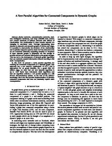
V. Experiments For the experiments we used a computing node of Hopper, a Cray XE6 distributed memory parallel computer. The node has 2 twelve-core AMD ‘MagnyCours’ 2.1-GHz processors and 32 GB DDR3 1333-MHz memory. Each core has its own L1 and L2 caches, with 64 KB and 512 KB, respectively. One 6-MB L3 cache is shared between 6 cores on the MagnyCours processor. All algorithms were implemented in C using OpenMP and compiled with gcc. Our test data set consists of four types of image data set: Texture, Aerial, Miscellaneous and NLCD. First three data sets are taken from the image database of the University of Southern California.1 The fourth data set is taken from US National Cover Database 2006.2 All of the images are converted to binary images by MATLAB using im2bw(level) function with level value as 0.5. The function converts the grayscale image to a binary image by replacing all pixels in the input image with luminance greater than 0.5 with the value 1 (white) and replaces all other pixels with the value 0 (black). If the input image is not a grayscale image, im2bw converts the input image to grayscale, and then converts this grayscale image to binary(Figure 3). However, note that our algorithm can be easily extended to gray scale images. Texture, Aerial and Miscellaneous data set contain images of size 1 MB or less. NCLD data set contains images of size bigger than 12 MB. The biggest image in the data set is 465.20 MB. Firstly, we performed the experiment over all the sequential algorithms. The experimental results are shown in Table II. In the table, we have shown the minimum, maximum and average execution time of all the four data sets. The execution time of AR EM SP is lowest among all the sequential algorithms. Thus AR EM SP is best among all the sequential algorithms. Next, we show our results for the parallel algorithm 1 http://sipi.usc.edu/database/ 2 http://dx.doi.org/10.1016/j.cageo.2013.05.014
6 TABLE II: Comparison of various execution times[msec] for sequential algorithms
Image type Aerial
Texture
Misc (a) Original Image
(b) Binary Image NLCD
Fig. 3: Example of color image to binary image
10
CCLRemSP 2.48 13.25 80.90 2.06 8.20 16.18 0.49 3.21 12.81 4.46 299.55 1273.82
ARun 1.98 11.90 72.92 1.58 7.32 14.81 0.36 2.75 11.30 3.77 244.88 1036.52
ARemSP 1.95 11.86 70.17 1.53 7.27 14.47 0.36 2.74 11.20 3.75 242.59 1021.45
TABLE III: Images and their sizes [in MB]
Aerial Miscellaneous Texture
Image name image 1 image 2 image 3 image 4 image 5 image 6
8 Speedup
CCLLRPC 2.5 13.68 86.64 2.07 8.42 16.86 0.50 3.28 12.96 4.61 307.66 1307.27
Min Average Max Min Average Max Min Average Max Min Average Max
6 4
Size 12 33 37.31 116.30 132.03 465.20
TABLE IV: Execution time [msec] of PAR EM SP algorithm for various # threads
Image type Aerial
2
2
6
8 #Threads
16
24
Fig. 4: Speedup for different images and different numbers of threads for Aerial, Texture & Miscellaneous data set
PAR EM SP over all the images. We have shown the speedup for data sets (except NCLD image data set) in Figure 4. The minimum, maximum and average execution time of PAR EM SP for all the datasets is also shown in Table IV. We get a maximum speedup of 10 in this case as the images are 1 MB or less in size. The speedup also decreases in some cases as the number of threads increases. This case occurs when the image size is small. As the number of threads increase, each threads has less work, and therefore the thread creation and termination overhead will affect the performance. Figure 5a-5b shows the speedup of the algorithm for NCLD image data set. The size of the images are given in Table III. We get a maximum speedup of 20.1 on 24 cores for image of size 465.20 MB. Figure 5a shows the speedup for Phase-I of PAR EM SP i.e. the local computation and Figure 5b shows the overall speedup (i.e. local + merge). We can see that there is not significant difference between both speedups, implying that merge operation does not have a significant overhead. Also Figure 5 shows, speedup increases with image size. Therefore, our parallel implementation is able to achieve near linear speed for large data sets.
VI. Conclusion In this paper, we presented two sequential CCL algorithms CCLR EM SP and AR EM SP which are based on union-find technique of R EM ’s algorithm and scan strategies of ARUN
Min Average Max
2 1.39 7.92 46.86
6 0.84 3.03 16.72
16 1.02 1.87 7.32
24 1.38 2.15 6.97
Texture
Min Average Max
1.09 4.91 9.75
0.62 1.99 3.56
0.93 1.45 2.11
1.36 1.82 2.34
Miscellaneous
Min Average Max
0.36 1.99 7.96
0.36 0.97 3.24
0.79 1.05 1.91
1.18 1.46 2.27
NLCD
Min Average Max
2.52 162.86 676.41
1.16 58.50 184.71
1.32 20.20 78.33
1.67 13.47 51.00
and CCLLRPC algorithms. CCLR EM SP algorithm uses the scan strategy of CCLLRPC algorithm whereas AR EM SP uses the scan strategy of ARUN algorithm. Based on the experiments, we found out that AR EM SP outperforms all the other sequential algorithms. We also implement a portable parallel implementation of AR EM SP for shared memory computers with standard OpenMP directives. Our proposed algorithm, PAR EM SP, divides the image into equal proportions and executes the scan. To merge the provisional labels on the image boundary, we use the parallel version of R EM ’s algorithm. Our experimental results conducted on a shared memory computer show scalable performance, achieving speedups up to a factor of 20.1 when using 24 cores on data set of size 465.20 MB. Thus, our parallel algorithm achieves linear scaling for large fixed problem size while the number of processing elements are increased.
Acknowledgment This work is supported in part by the following grants: NSF awards CCF-0833131, CNS-0830927, IIS-0905205, CCF-0938000, CCF-1029166, ACI-1144061, and IIS-1343639; DOE awards DE-FG02-08ER25848, DE-SC0001283,
25
25
20
20
15
15
Speedup
Speedup
7
10
10 5
5
0
0 0
5
10
15
20
25
0
5
10
# Threads image 2
20
25
# Threads
(a) local
image 1
15
(b) local + merge
image 3
image 4
image 5
image 6
ideal
Fig. 5: Speedup for different images and different numbers of threads for NLCD data set
DE-SC0005309, DESC0005340, and DESC0007456; AFOSR award FA9550-12-1-0458.
[15]
References [1] Hussein M Alnuweiri and Viktor K Prasanna. Parallel architectures and algorithms for image component labeling. IEEE Transactions on Pattern Analysis and Machine Intelligence, 14(10):1014–1034, 1992. [2] Rafael C Gonzales and RE Woods. Digital image processing, 1993. [3] Pankaj K Agarwal, Lars Arge, and Ke Yi. I/o-efficient batched union-find and its applications to terrain analysis. In Proceedings of the twenty-second annual symposium on Computational geometry, pages 167–176. ACM, 2006. [4] Fu Chang, Chun-Jen Chen, and Chi-Jen Lu. A linear-time component-labeling algorithm using contour tracing technique. Computer Vision and Image Understanding, 93(2):206–220, 2004. [5] Hiroki Hayashi, Mineichi Kudo, Jun Toyama, and Masaru Shimbo. Fast labelling of natural scenes using enhanced knowledge. Pattern Analysis & Applications, 4(1):20–27, 2001. Fast [6] Qingmao Hu, Guoyu Qian, and Wieslaw L Nowinski. connected-component labelling in three-dimensional binary images based on iterative recursion. Computer Vision and Image Understanding, 99(3):414–434, 2005. [7] Felipe Knop and Vernon Rego. Parallel labeling of three-dimensional clusters on networks of workstations. Journal of Parallel and Distributed Computing, 49(2):182–203, 1998. [8] Alina N Moga and Moncef Gabbouj. Parallel image component labelling with watershed transformation. Pattern Analysis and Machine Intelligence, IEEE Transactions on, 19(5):441–450, 1997. [9] Kuang-Bor Wang, Tsorng-Lin Chia, Zen Chen, and Der-Chyuan Lou. Parallel execution of a connected component labeling operation on a linear array architecture. J. Inf. Sci. Eng., 19(2):353–370, 2003. [10] Kenji Suzuki, Isao Horiba, and Noboru Sugie. Linear-time connected-component labeling based on sequential local operations. Computer Vision and Image Understanding, 89(1):1–23, 2003. [11] RM Haralick. Some neighborhood operators. In Real-Time Parallel Computing, pages 11–35. Springer, 1981. [12] A Hashizume, R Suzuki, H Yokouchi, H Horiuchi, and S Yamamato. An algorithm of automated rbc classification and its evaluation. Bio Medical Engineering, 28(1):25–32, 1990. [13] Toshiyuki Gotoh, Yoshiyuki Ohta, Masumi Yoshida, and Yoshiaki Shirai. High-speed algorithm for component labeling. Systems and Computers in Japan, 21(5):74–84, 1990. [14] Toshiyuki Gotoh, Yoshiyuki Ohta, Masumi Yoshida, and Yoshio Shirai. Component labeling algorithm for video rate processing. In Hague
[16]
[17]
[18]
[19] [20] [21] [22]
[23]
[24] [25] [26]
[27]
[28]
[29]
[30]
International Symposium, pages 217–224. International Society for Optics and Photonics, 1987. Masatoshi Komeichi, Yoshiyuki Ohta, Toshiyuki Gotoh, Toshiya Mima, and Masumi Yoshida. Video-rate labeling processor. In 1988 Intl Congress on Optical Science and Engineering, pages 69–76. International Society for Optics and Photonics, 1989. Ronald Lumia. A new three-dimensional connected components algorithm. Computer Vision, Graphics, and Image Processing, 23(2):207–217, 1983. Ronald Lumia, Linda Shapiro, and Oscar Zuniga. A new connected components algorithm for virtual memory computers. Computer Vision, Graphics, and Image Processing, 22(2):287–300, 1983. Satoshi Naoi. High-speed labeling method using adaptive variable window size for character shape feature. In IEEE Asian Conference on computer vision, volume 1, pages 408–411, 1995. Azriel Rosenfeld. Connectivity in digital pictures. Journal of the ACM (JACM), 17(1):146–160, 1970. Azriel Rosenfeld and John L Pfaltz. Sequential operations in digital picture processing. Journal of the ACM (JACM), 13(4):471–494, 1966. Y Shirai. Labeling connected regions. Three-Dimensional Computer Vision, pages 86–89, 1987. Michael B Dillencourt, Hannan Samet, and Markku Tamminen. A general approach to connected-component labeling for arbitrary image representations. Journal of the ACM (JACM), 39(2):253–280, 1992. Irene Gargantini and Zale Tabakman. Separation of connected component using linear quad-and oct-trees. In Proc. 12th Conf. Numerical Mathematics and Computation, volume 37, pages 257–276, 1982. Jean Hecquard and Raj Acharya. Connected component labeling with linear octree. Pattern recognition, 24(6):515–531, 1991. Hanan Samet. Connected component labeling using quadtrees. Journal of the ACM (JACM), 28(3):487–501, 1981. Hanan Samet and Markku Tamminen. Computing geometric properties of images represented by linear quadtrees. Pattern Analysis and Machine Intelligence, IEEE Transactions on, (2):229–240, 1985. Hanan Samet and Markku Tamminen. Efficient component labeling of images of arbitrary dimension represented by linear bintrees. Pattern Analysis and Machine Intelligence, IEEE Transactions on, 10(4):579–586, 1988. Hanan Samet and Markku Tamminen. An improved approach to connected component labeling of images. In International Conference on Computer Vision And Pattern Recognition, pages 312–318, 1986. Markku Tamminen and Hanan Samet. Efficient octree conversion by connectivity labeling. In ACM SIGGRAPH Computer Graphics, volume 18, pages 43–51. ACM, 1984. Prabir Bhattacharya. Connected component labeling for binary images
8
[31] [32] [33] [34] [35] [36] [37] [38]
[39] [40] [41] [42]
[43]
on a reconfigurable mesh architecture. Journal of Systems Architecture, 42(4):309–313, 1996. Alok Choudhary and Rajeev Thakur. Connected component labeling on coarse grain parallel computers: an experimental study. Journal of Parallel and Distributed Computing, 20(1):78–83, 1994. Daniel S. Hirschberg, Ashok K. Chandra, and Dilip V. Sarwate. Computing connected components on parallel computers. Communications of the ACM, 22(8):461–464, 1979. M Manohar and HK Ramapriyan. Connected component labeling of binary images on a mesh connected massively parallel processor. Computer vision, graphics, and image processing, 45(2):133–149, 1989. David Nassimi and Sartaj Sahni. Finding connected components and connected ones on a mesh-connected parallel computer. SIAM Journal on computing, 9(4):744–757, 1980. Stephan Olariu, James L Schwing, and Jingyuan Zhang. Fast component labelling and convex hull computation on reconfigurable meshes. Image and vision computing, 11(7):447–455, 1993. Kesheng Wu, Ekow Otoo, and Kenji Suzuki. Optimizing two-pass connected-component labeling algorithms. Pattern Analysis and Applications, 12(2):117–135, 2009. Lifeng He, Yuyan Chao, and Kenji Suzuki. A new two-scan algorithm for labeling connected components in binary images. In Proceedings of the World Congress on Engineering, volume 2, 2012. Md Patwary, Mostofa Ali, Peder Refsnes, and Fredrik Manne. Multi-core spanning forest algorithms using the disjoint-set data structure. In Parallel & Distributed Processing Symposium (IPDPS), 2012 IEEE 26th International, pages 827–835. IEEE, 2012. Chien-Wei Chen, Yi-Ta Wu, Shau-Yin Tseng, and Wen-Shan Wang. Parallelization of connected-component labeling on tile64 many-core platform. Journal of Signal Processing Systems, pages 1–15, 2013. Md Mostofa Ali Patwary, Jean Blair, and Fredrik Manne. Experiments on union-find algorithms for the disjoint-set data structure. In Experimental Algorithms, pages 411–423. Springer, 2010. Edsger Wybe Dijkstra, Edsger Wybe Dijkstra, Edsger Wybe Dijkstra, and Edsger Wybe Dijkstra. A discipline of programming, volume 1. prentice-hall Englewood Cliffs, 1976. Mehdi Niknam, Parimala Thulasiraman, and Sergio Camorlinga. A parallel algorithm for connected component labelling of gray-scale images on homogeneous multicore architectures. In Journal of Physics: Conference Series, volume 256, page 012010. IOP Publishing, 2010. Lifeng He, Yuyan Chao, and Kenji Suzuki. A run-based two-scan labeling algorithm. Image Processing, IEEE Transactions on, 17(5):749–756, 2008.