May 9, 2008 - while demonstating their flaws. In Section 3 we derive our new algorithm which attempts to overcome these. Section 4 contains a simulation ...
A Sequential Smoothing Algorithm with Linear Computational Cost Paul Fearnhead
David Wyncoll
Jonathan Tawn
May 9, 2008 Abstract In this paper we propose a new particle smoother that has a computational complexity of O(N ), where N is the number of particles. This compares favourably with the O(N 2 ) computational cost of most smoothers and will result in faster rates of convergence for fixed computational cost. The new method also overcomes some of the degeneracy problems we identify in many existing algorithms. Through simulation studies we show that substantial gains in efficiency are obtained for practical amounts of computational cost. It is shown both through these simulation studies, and on the analysis of an athletics data set, that our new method also substantially outperforms the simple FilterSmoother (the only other smoother with computational cost that is linear in the number of particles).
1
Introduction
State space models provide a flexible framework to handle non-linear time series. These models assume a time-series with observations Yt that are conditionally independent given a hidden Markov process Xt . Formally the model is given by a state equation and an observation equation, which can be represented in terms of conditional distributions Xt+1 |{X1:t = x1:t , Y1:t = y1:t } ∼ f (·|xt ), Yt |{X1:t = x1:t , Y1:t−1 = y1:t−1 } ∼ g(·|xt ), where we use the notation that x1:t = (x1 , . . . , xt ), and similarly for y1:t . The model is completed through specifying an initial distribution for X0 . When the observations are arriving sequentially we are often interested in the current value of the state Xt given all the available data. For this filtering problem, interest lies in estimating the posterior distribution p(xt |y1:t ). Sequential Monte Carlo algorithms, known generically as particle filters, have recently emerged as a solution to this problem. These filters approximate p(xt |y1:t ) by a set of N weighted particles; and are based on steps for sequentially producing a set of weighted particles that approximate p(xt |y1:t ) given a set that approximates p(xt−1 |y1:t−1 ). In their simplest form these algorithms produce equally weighted particles, and the particles can be viewed as an approximate sample from p(xt |y1:t ) (see Gordon et al. (1993) or Kitagawa (1996)). The computational complexity of particle filters is usually linear in the number of particles, 1
N , and as such large numbers of them can be chosen to best approximate the target posterior. Our interest in this paper lies in the related smoothing problem whose aim is to obtain estimates of previous states given a block of observations y1 , . . . , yT . While this problem can be theoretically solved with a slight modification of the particle filter (see Kitagawa (1996)), it is easy to show that this produces a poor approximation of the smoothing density p(xt |y1:T ) for t � T . With this in mind, alternative algorithms to sequentially approximate p(xt |y1:T ) after a particle filter have been developed (see for example Kitagawa (1996), H¨ urzeler and K¨ unsch (1998), Doucet et al. (2000), Godsill et al. (2004) and Briers et al. (2004)). All these methods involve a step to re-weight particles that approximate a filter distribution so that the re-weighted particles approximate p(xt |y1:T ). While they perform comparably well for a fixed number of particles, N , these algorithms have a complexity of O(N 2 ) and therefore their use is restricted to smaller N than is used for particle filtering. Also, for some state-space models, particularly those for which a component of Xt is uniquely determined by the previous state, xt−1 , these alternative smoothing algorithms can degenerate; either they become equivalent to the O(N ) smoother of Kitagawa (1996) or cannot be applied at all. We present a new smoothing algorithm. The basic idea is to allow the smoother to simulate new particles which will be used to approximate p(xt |y1:T ), rather than just re-weighting existing particles. This approach avoids some of the degeneracy issues of existing particle smoothers. However, the most important feature of our new smoothing algorithm is that there is a set of models for which the computational complexity is linear in the number of particles. This set includes all models with a linear-Gaussian state equation, and all models for which the likelihood, g(yt |xt ) is integrable in xt . This covers a wide-variety of models such as the bearings-only tracking model (Gordon et al., 1993), factor stochastic volatility models (Liu and West, 2001), time varying auto-regressive coefficient models (Kitagawa and Gersch, 1985) and ARCH models (Fearnhead, 2005) amongst many others. Our work itself was motivated by problems of non-stationarity when modelling the extremes of a time-series. For example, in Section 5, we consider data on the fastest times for the women’s 3000m (see Figure 4). Whilst up to 1982 there is evidence of a year-on-year improvement in times for this event, since 1982 times have plateaued – if anything times worsened in the latter half of the 1980s, perhaps due to increased regulation and testing for the use of performance enhancing drugs. It is natural to model the data from each year using a distribution which is motivated by asymptotic extreme value theory; and we incorporate non-stationarity into this distribution through allowing its location parameter to vary in a non-parametric way. We can thus obtain a state-space model for the data, where the state is the location parameter. Standard nonparametric models, such as random walks and integrated random walks, can be formulated as linear-Gaussian models for the location parameter. See Smith and Miller (1986) for an example of state space models being used to analyse athletics records. The article is organised as follows. We begin Section 2 by describing particle filtering and go on to review the current methods for sequential smoothing while demonstating their flaws. In Section 3 we derive our new algorithm which attempts to overcome these. Section 4 contains a simulation study with a mul2
tivariate Normal model, which shows the substantial improvements our new smoother gives for models with a linear-Gaussian state equation. Section 5 compares relative efficiencies of the methods at analysing the athletics dataset, and addresses the question as to how extreme the 1993 world record of Wang Junxia was. To analyse these data, we develop an efficient EM algorithm that utilises our new smoother, to estimate fixed parameters in the extreme value distribution. Our analysis suggests that a new world record as or more extreme as that of Wang Junxia’s would happen less than once every 5000 years from the evidence about the population of the other top athletes in this event.
2 2.1
Current methods for particle smoothing Particle filtering
The aim of Bayesian filtering is to calculate sequentially the filter distributions p(xt |y1:t ) upon receipt of observations yt . The analytical solution to this problem is given by Z p(xt |y1:t ) ∝ g(yt |xt ) f (xt |xt−1 )p(xt−1 |y1:t−1 ) dxt−1 , (1) which relates p(xt |y1:t ) to p(xt−1 |y1:t−1 ) and yt . This recursion is intractable in general, although an important exception to this is when both the state f and the likelihood g are linear-Gaussian densities and the prior is also Gaussian. In this case the solution is given by the Kalman filter recursions of Kalman (1960). Particle filters aim to overcome the intractability of (1) by using potential draws of the state to approximate the unknown filter distributions. In general, we approximate the distribution p(xt |y1:t ) by a discrete distribution with sup(i) (i) N port {xt }N i=1 and probability masses {wt }i=1 . Applying this to p(xt−1 |y1:t−1 ) in (1) gives the approximation p(xt |y1:t ) ' cg(yt |xt )
N X
(i)
(i)
f (xt |xt−1 )wt−1 ,
(2)
i=1
where c is a normalising constant. A particle filter algorithm gives steps for producing weighted particles to approximate this. For reviews of various filtering methods see for example Liu and Chen (1998), Doucet et al. (2000) and Fearnhead (2008). We focus our attention on the auxiliary particle filter of Pitt and Shephard (1999). This is a general method through which many simpler particle filters can be defined as special cases. In this approach we aim to approximate (i)
(i)
cg(yt |xt )f (xt |xt−1 )wt−1
(3)
by (i)
(i)
q(xt |xt−1 , yt )βt , (i)
(i)
where q(·|xt−1 , yt ) is a distribution we can sample from and {βt }N i=1 are normalised weights which sum to 1. We then use a combination of re-sampling and importance sampling to generate a weighted sample approximating (2). 3
Algorithm 1 gives the general algorithm for sequentially sampling weighted (i) (i) particles {(xt , wt )} approximating p(xt |y1:t ). While the simplest way to initialise the algorithm is to sample from the prior p(x0 ) and propagate from t = 1, it is usually possible and more accurate to sample from p(x1 |y1 ) directly using standard importance sampling. Algorithm 1 Auxiliary particle filter of Pitt and Shephard (1999) (i)
(i)
1. Initialisation: Sample {x0 } from the prior p(x0 ) and set w0 = 1/N for all i. 2. For t = 1, 2, . . . (i)
(a) Re-sample: Use the {βt } as probabilities to sample N indices j1 , ..., jN from {1, ..., N }. (i)
(b) Propagate: Sample the new particles xt independently from (ji ) q(·|xt−1 , yt ). (i)
(c) Re-weight: Assign each particle xt the corresponding importance weight (ji ) (i) (ji ) (i) )wt−1 g(yt |xt )f (xt |xt−1 (i) wt ∝ (j ) (i) (ji ) , yt )βt i q(xt |xt−1 and normalise them to sum to 1.
The efficiency of the particle filter rests primarily on the choice of proposal (i) density q and re-sampling weights βt . In the simplest case we could have (i) (i) q(xt |xt−1 , yt ) = f (xt |xt−1 ) and βt = wt−1 which is essentially the algorithm of Gordon et al. (1993). Such a choice would place mass unevenly on the particles thus wasting those with small weights. To rectify this the auxiliary approach (i) produces more even weights if q and βt are chosen so that (3) is well approxi(i) (i) (i) (i) (i) mated. In particular if q(xt |xt−1 , yt ) = p(xt |xt−1 , yt ) and βt ∝ p(yt |xt−1 )wt−1 (i) then the final weights wt will all equal 1/N and we say the filter is adapted. (i) In most cases this optimal choice of q and βt is not possible, but we can still obtain and use good approximations to them. Many authors have suggested further enhancements to the standard particle filter. The re-sampling step is optional and can be omitted by setting ji = (i) i thus propagating each particle xt−1 once. This eliminates any extra noise from re-sampling but gives uneven weights. Liu and Chen (1995) propose a measure of the effective sample size and resample only when it falls below a fixed threshold. Carpenter et al. (1999) show that the re-sampling noise is minimised by producing a stratified sample of the indices ji and give an O(N ) algorithm to achieve this. A further enhancement which takes advantage of the linear-Gaussian state is Rao-Blackwellisation; see Casella and Robert (2001) for an introduction to the topic and Doucet et al. (2000) for an application to particle filtering. The idea is that for some models it is possible to integrate out part of the state analytically. This enables the integrable part of the state to be represented by a distribution 4
rather than a specific value. The advantage of Rao-Blackwellisation is that less Monte Carlo error is accrued in each update and so the variance of estimates is reduced. An example of the application of Rao-Blackwellisation is given in Section 5.
2.2
Smoothing while filtering
In its simplest form, smoothing can be achieved from a simple extension to the particle filter as shown by Kitagawa (1996), and we call the resulting algorithm the Filter-Smoother. As with the filter distribution p(xt |y1:t ) in (1), we have a recursive solution for the joint smoothing distribution: p(x1:t |y1:t ) ∝ g(yt |xt )f (xt |xt−1 )p(x1:t−1 |y1:t−1 ).
(4)
By comparing (1) and (4) it is easy to show that the particle filter steps can (i) (i) be used to update weighted paths {(x1:t , wt )}N i=1 approximating p(x1:t |y1:t ). Doing so simply requires keeping track of the inheritance of the newly sampled (i) (ji ) (i) (i) , xt ). This means that any filtering algoparticle xt by setting x1:t = (x1:t−1 rithm can be used and the method inherits the O(N ) computational complexity of the filter making large numbers of particles feasible. While this Filter-Smoother approach can produce an accurate approximation of the filtering distribution p(xt |y1:t ) it gives a poor representation of previous (i) states. To see this we note that whenever we resample the paths {x1:t−1 } by sampling the auxiliary variables {ji } we end up with multiple copies of some paths but lose others altogether. Therefore the number of distinct particles at any given time decreases monotonically the more times we resample. Also, with multiple copies of some particles, their weights are effectively added together on a single point so that marginally the weights become more uneven as we look back in time. 1
2
3
4
5
6
●
●
●
●
●
●
●
●
●
●
●
●
●
●
●
●
●
●
●
●
●
●
●
●
●
●
●
●
● ●
●
●
●
● ●
●
●
●
●
●
●
●
●
●
●
●
●
●
●
●
●
●
●
●
●
●
Figure 1: Plot showing how the simple smoother re-weights filter particles. The arrows represent the dependencies between the particles at time t and t − 1 due to re-sampling. The size of the particle represents its total weight as a draw from the smoothed distribution. 5
(i)
This can be seen in Figure 1 which represents 10 smoothed paths x1:6 showing how they re-weight filter particles. As you can see, particles which are lost due to re-sampling receive no weight and particles with many offspring have large weights. While the filter approximation at time 6 is good, the weights become more uneven as the number of weighted particles decreases going back in time. This is not surprising since the particles at times t < 6 are drawn to approximate p(xt |y1:t ) so must be unevenly weighted if they are to represent a different distribution. As a final point we note that re-sampling more infrequently can improve this method of smoothing although there is a limit to how much this can help. Even with no re-sampling, the approximation to p(xt |y1:T ) will deteriorate as T − t gets large: with the particle approximation tending to give non-negligible weight to all but a small subset of particles, and eventually only one particle having a non-negligible weight.
2.3
Other smoothing algorithms
Several algorithms have been proposed to improve on the simple Filter-Smoother. A common requirement is that a particle filter is run first to give weighted par(i) (i) ticles {(xt , wt )}N i=1 approximating p(xt |y1:t ) for t = 1, . . . , T . 2.3.1
Forward-Backward smoothing
The Forward-Backward Smoother of Doucet et al. (2000), as well as the related algorithms of Tanizaki and Mariano (1994) and H¨ urzeler and K¨ unsch (1998), is based around the backwards recursion Z f (xt+1 |xt ) p(xt+1 |y1:T ) dxt+1 , for t < T . p(xt |y1:T ) = p(xt |y1:t ) p(xt+1 |y1:t ) The unknown densities can be approximated using filter particles from the current time t and smoother particles from t + 1 to obtain p(xt |y1:T ) '
N X
(i)
(i)
δ(xt − xt )wt|T ,
i=1
where (i) wt|T
:=
(j)
N X j=1
(i)
(i)
f (xt+1|T |xt )wt PN
(j)
(k)
(j)
(k)
k=1 f (xt+1|T |xt )wt
wt+1|T
(5)
and δ(·) is the Dirac delta function. This approximation can be used to sequentially re-weight the filter particles backwards in time so that they represent the marginal smoothing densities. 2.3.2
Two-Filter smoothing
The Two-Filter Smoother of Briers et al. (2004) combines samples from a particle filter with those from a backwards information filter to produce estimates of p(xt |y1:T ).
6
The backwards information filter produces sequential approximations of the likelihood p(yt:T |xt ) backwards through time and is based on the following recursion: Z p(yt:T |xt ) = g(yt |xt ) f (xt+1 |xt )p(yt+1:T |xt+1 ) dxt+1 , for t < T . (6) Since p(yt:T |xt ) is not a probability density function in xt it may not have a finite integral over xt in which case a particle representation will not work. The smoothing algorithm in Kitagawa (1996) assumes implicitly that this is not the case but Briers et al. (2004) propose the following construction which will always give a finite measure. They introduce an artificial prior distribution γ0 (x0 ) which, when substituted for p(x0 ), yields a backwards filter density p˜(xt |yt:T ) ∝ γt (xt )p(yt:T |xt ),
(7)
R
where γt (xt ) = f (xt |xt−1 )γt−1 (xt−1 ) dxt−1 is derived recursively from γ0 (x0 ). An artificial prior is introduced so that γt (xt ) is available in closed form which is only possible when the state is linear-Gaussian. If the prior p(x0 ) is also Gaussian then this can be used instead of γ0 (x0 ). If however the state is not linear-Gaussian but the likelihood g(yt |xt ) is integrable, we can instead propagate a particle representation of p(yt:T |xt ) by assuming γt (xt ) ≡ 1 throughout the following derivation. Following on from (6) the backwards filter is derived from Z p˜(xt+1 |yt+1:T ) dxt+1 p˜(xt |yt:T ) ∝ γt (xt )g(yt |xt ) f (xt+1 |xt ) γt+1 (xt+1 ) ' γt (xt )g(yt |xt ) (k)
(k) N X f (˜ xt+1 |xt ) (k) xt+1 ) k=1 γt+1 (˜
(k)
w ˜t+1 ,
(k)
where the weighted particles {(˜ xt+1 , w ˜t+1 )} approximate p˜(xt+1 |yt+1:T ). This is very similar to the derivation of the forwards filter and as such many filtering algorithms and enhancements can be modified for this purpose. For example, an auxiliary backwards filter in the style of Pitt and Shephard (k) (1999) can be made by finding a distribution q˜(·|yt , x ˜t+1 ) we can sample from such that (k)
(k) (k) (k) xt+1 |xt ) ˜t+1 )β˜t ' γt (xt )g(yt |xt )f (˜ q˜(xt |yt , x
w ˜t+1 (k)
.
xt+1 ) γt+1 (˜
We then proceed analogously to Algorithm 1 for t = T, ..., 1 after initialising the algorithm with particles drawn from γT +1 (xT +1 ). An adapted backwards filter (k) (k) (k) giving even weights w ˜t = 1/N is achieved with q˜(xt |yt , x ˜t+1 ) = p(xt |yt , x ˜t+1 ) (k) (k) (k) and β˜t ∝ p˜(yt |˜ xt+1 )w ˜t+1 where we again use p˜ to denote a distribution which uses γ0 (x0 ) as the prior instead of p(x0 ). Having run a forwards particle filter and a backwards information filter, it is possible to combine the two to estimate p(xt |y1:T ). The Two-Filter Smoother is based upon writing the target density as p(xt |y1:T ) ∝ p(xt |y1:t−1 ) · p(yt:T |xt ) Z p˜(xt |yt:T ) ∝ f (xt |xt−1 )p(xt−1 |y1:t−1 ) dxt−1 · . γt (xt ) 7
(j)
(j)
Therefore filter particles {(xt−1 , wt−1 )} approximating p(xt−1 |y1:t−1 ) and back(k) (k) wards filter particles {(˜ xt , w ˜t )} approximating p˜(xt |yt:T ) are used to obtain p(xt |y1:T ) '
N X
(k)
(k)
δ(xt − x ˜t )w ˜t|T ,
k=1
where (k)
(k)
w ˜t|T :∝
w ˜t
N X
(k) γt (˜ xt ) j=1
(k)
(j)
(j)
f (˜ xt |xt−1 )wt−1 .
(8)
Thus particles from a forwards filter are used to re-weight those from a backwards filter so that they represent the target distribution.
2.4
Comparison of current particle smoothers
Both the Forward-Backward and Two-Filter smoothers aim to improve on the simple Filter-Smoother by removing its dependence on the inheritance paths of the particle filter. Forward-Backward smoothing does this by reweighting the filter particles while Two-Filter smoothing re-weights particles sampled from a backwards filter. However, both algorithms are O(N 2 ) as the calculation of each particle’s weight is an O(N ) operation1 . Thus, while variants of these particle smoothers produce better estimates for a fixed particle number N , far fewer particles can be used for these algorithms than can for the Filter-Smoother in a fixed amount of time. Another advantage of the Filter-Smoother is that it gives draws of the joint smoothing distribution p(x1:T |y1:T ) rather than only the marginal distributions. It is possible to adapt the Forward-Backward Smoother to also draw samples from the joint smoothing distribution as shown in H¨ urzeler and K¨ unsch (1998) and Godsill et al. (2004). Their derivation is similar to that of the ForwardBackward Smoother above and as such share its complexity and are determined by the re-sampling of the filter. They therefore achieve better samples of the joint distribution than the Filter-Smoother for a fixed N but give a slightly worse representation of the marginal distributions than the Forward-Backward Smoother. Since the Forward-Backward Smoother and the Filter-Smoother rely on the support of filter particles we may expect them to approximate p(xt |y1:T ) best for t close to T where the target is most similar to p(xt |y1:t ). Likewise the TwoFilter Smoother may do best for small t when the backwards filter distribution p˜(xt |yt:T ) is likely to be closest to our target. However when there is a large discrepancy between these distributions the particles will be weighted very unevenly as they will not be located in the right position to represent the smoothed distribution. Ideally we would like an algorithm which samples particles in the correct position for the smoothed distribution. 1 The overall cost of calculating the weight (5) in the Forward-Backward Smoother is O(N ) as each of the terms in the denominator need to be calculated only once and can then be stored
8
2.5
Degeneracy of the Forward-Backward and Two-Filter smoothers
As a final point we note that the Forward-Backward and Two-Filter smoothers’ reliance on the form of the state density causes degeneracy problems with certain models and filters. Specifically, this happens whenever f (xt |xt−1 ) is zero or approximately so for most combinations of possible xt and xt−1 . As an example, consider the simple AR(2) process zt = φ1 zt−1 + φ2 zt−2 + �t with �t ∼ N (0, ν 2 ). The model can be written as a two-dimensional Markov 0 process by defining the state as xt = (xt,1 , xt,2 ) where xt,1 = zt and xt,2 = zt−1 . This gives the state transition density f (xt |˜ xt−1 ) = N (xt,1 |φ1 x ˜t−1,1 + φ2 x ˜t−1,2 , ν 2 ) δ(xt,2 − x ˜t−1,1 ), where we write N (z|µ, ν 2 ) for the density of N (µ, ν 2 ) evaluated at z. This density is zero whenever the second component of xt does not equal the first (i) (j) component of x ˜t−1 . This means that for two sets of particles {˜ xt−1 } and {xt }, (i) (j) (i) (j) f (xt |˜ xt−1 ) is likely to be zero unless xt was generated from x ˜t−1 . Since the Forward-Backward Smoother relies on comparing particles sampled from the filter at time t with those at time t + 1, it can be shown that the weight (5) reduces to the effective weight given to each particle by the Filter-Smoother. However the situation is worse for Two-Filter smoothing which fails completely as the forwards and backwards filter particles were sampled independently. With probability 1, no pairs of forwards and backwards filter particles match and so all the weights (8) will be zero.
3
New smoothing algorithm
We now describe our new smoothing algorithm which attempts to overcome the weaknesses of the current methods. Our primary aim is to draw new particles from the marginal smoothing densities directly rather than re-weight those drawn from another distribution. We describe the basic idea first, and then look at how the smoother can be implemented so that its computational cost is linear in the number of particles. We start with a similar derivation to the Two-Filter Smoother which gives p(xt |y1:T ) ∝ p(xt |y1:t−1 ) · g(yt |xt ) · p(yt+1:T |xt ) Z ∝ f (xt |xt−1 )p(xt−1 |y1:t−1 ) dxt−1 · g(yt |xt )· Z p˜(xt+1 |yt+1:T ) f (xt+1 |xt ) dxt+1 , γt+1 (xt+1 ) where we use the artificial prior and backwards filter in (7) above. These integrals can be approximated using weighted particles from a particle filter at time t − 1 and from a backwards information filter at time t + 1 to obtain p(xt |y1:T ) ' c
N X N X
(k)
(j) (j) f (xt |xt−1 )wt−1
j=1 k=1
9
· g(yt |xt ) ·
f (˜ xt+1 |xt ) (k) γt+1 (˜ xt+1 )
(k)
w ˜t+1 ,
(9)
where c is a normalising constant. Though this formula can be written as the product of two sums, we write it as a double sum to emphasise that there are N 2 (j, k) pairs. We also note that any filtering algorithm can be used to generate (j) (k) {xt−1 } and {˜ xt+1 } as long as the artificial prior γt+1 (xt+1 ) here is the same one (k) (k) used to sample {(˜ xt+1 , w ˜t+1 )} in the backwards information filter. As before we assume γt+1 (xt+1 ) ≡ 1 throughout if the backwards filter approximates p(yt+1:T |xt+1 ) instead of p˜(xt+1 |yt+1:T ). To sample from this approximation we start by mirroring the auxiliary particle filter of Pitt and Shephard (1999) by finding a sampling distribution q¯ and (j,k) such that weights β¯t (j)
(k)
w w ˜t+1 (j) (k) (j,k) (j) (k) q¯(xt |xt−1 , yt , x ˜t+1 )β¯t ' f (xt |xt−1 )g(yt |xt )f (˜ xt+1 |xt ) t−1 (k) . γt+1 (˜ xt+1 ) (j,k) Algorithm 2 gives the algorithm that results from using the β¯t s to sample (i) (j, k) pairs before using q¯ to sample new particles x ¯t .
Algorithm 2 New O(N 2 ) smoothing algorithm (j)
(j)
1. Filter forwards: Run a particle filter to generate {(xt , wt )} approximating p(xt |y1:t ) for t = 0, . . . , T . 2. Filter backwards: Run a backwards information filter to generate (k) (k) {(˜ xt , w ˜t )} approximating p˜(xt |yt:T ) ∝ γt (xt )p(yt:T |xt ) for t = T, . . . , 2. 3. Smooth: For t = 1, . . . , T − 1 (j,k)
(a) Re-sample: Calculate the β¯t sample N pairs {(ji , ki )}N i=1 .
s and use them as probabilities to (i)
(b) Propagate: Sample the new particles x ¯t independently from (ji ) (ki ) ˜t+1 ). q¯(·|xt−1 , yt , x (i)
(c) Re-weight: Assign each particle x ¯t the weight (i)
(i)
w ¯t ∝
(j )
(i)
(k )
(i)
(j )
(k )
i i i i w ˜t+1 xt+1 |¯ xt ) wt−1 f (¯ xt |xt−1 ) g(yt |¯ xt ) f (˜ (ki ) (i) (ji ) (ki ) ¯(ji ,ki ) γt+1 (˜ xt+1 ) q¯(¯ xt |xt−1 , yt , x ˜t+1 ) βt
and normalise them to sum to 1. (j )
(i)
(k )
i i Note that the output of Algorithm 2 is a set of triples, (xt−1 ,x ¯t , x ˜t+1 ), (i) with associated weights, w ¯t . These can be viewed as a particle approximation to p(xt−1:t+1 |y1:T ). If our interest solely lies in the marginal p(xt |y1:T ) (i) (i) we just keep the particles, x ¯t , and their associated weights, w ¯t . We note (j) (k) ˜t+1 ) = further that the optimal choice of propagation density is q¯(xt |xt−1 , yt , x (j) (k) p(xt |xt−1 , yt , x ˜t+1 ) while the optimal re-sampling probabilities are given by
(j,k) β¯t ∝
Z
(j)
(j)
(k)
f (xt |xt−1 )g(yt |xt )f (˜ xt+1 |xt ) dxt
10
(k)
wt−1 w ˜t+1 (k)
γt+1 (˜ xt+1 )
.
(10)
We do not require our algorithm to generate samples for time T since these are available from the filter. Similarly, particles for time 1 are available from the backwards filter if we use γ0 (x0 ) = p(x0 ) for the artificial prior. Algorithm 2 overcomes the degeneracy problem of the Forward-Backward and Two-Filter smoothers when there is a deterministic relationship between the states at successive time-points, as demonstrated in Section 2.5 with the AR(2) model. Algorithm 2 will still have degeneracy problems where there is a deterministic relationship between components of states separated by two or more time-points. However it is simple, at least in theory, to extend our method (j) so that we jointly sample a block (xt , . . . , xt+n ) given filter particles {xt−1 } and (k) backwards filter particles {˜ xt+n+1 } (see Doucet et al. (2006) for an example of block sampling in particle filters). By choosing n sufficiently large such that there is not deterministic relationship between components of xt and xt+n , our approach to smoothing can then be applied in these cases. Like the Two-Filter Smoother in Section 2, our smoothing step is not sequential and can be performed independently for each time t. Also, the computational complexity of each step is O(N 2 ) which is comparable with all but the (j,k) simplest Filter-Smoother. However, as it stands we have N 2 β¯t s to calculate 2 making it O(N ) in memory also which could mean that it is impractical for even modest sample sizes.
3.1
Making Algorithm 2 O(N )
The above smoothing algorithm has a computational cost that is O(N 2 ), that is quadratic in the number of particles, due to the need to calculate N 2 prob(j,k) abilities, β¯t . A simple approach to reduce the computational cost of the smoothing algorithm is to choose these probabilities so that they correspond to choosing particles at time t − 1 and backward-filter particles at time t + 1 independently of each other. Our algorithm will then be O(N ) in computational complexity as well as memory and as such will be much faster for large N . Now the optimal distribution from which to choose the particles at time t−1 will be the corresponding marginal distribution of the optimal probabilities for (j,k) β¯t , given in (10). Marginalising we get: N X
(j,k) ∝ β¯t
k=1
N Z X
(j)
(j)
(k)
f (xt |xt−1 )g(yt |xt )f (˜ xt+1 |xt ) dxt
k=1
(k)
wt−1 w ˜t+1 (k)
γt+1 (˜ xt+1 )
(j) wt−1 p˜(xt+1 |yt+1:T ) (j) −−−−→ f (xt |xt−1 )g(yt |xt )f (xt+1 |xt ) dxt γt+1 (xt+1 ) (j) (j) ∝ p(yt:T |xt−1 )wt−1 . N →∞
ZZ
dxt+1
Calculating this analytically will be impossible, but it suggests two simple approximations. The first is to sample particles at time t − 1 according to their (j) filtering weights wt−1 . However a better approach will be to sample according (j) (j) to an approximation of p(yt |xt−1 )wt−1 , as it includes the information in the observation at time t. Now, in performing the particle filter we used the auxil(j) (j) iary filter which sampled particle xt−1 with a probability βt which is chosen (j) (j) to be an approximation to p(yt |xt−1 )wt−1 . Thus we suggest using exactly the 11
same probabilities to sample the particles within one iteration of our sampling algorithm. By similar calculations, it can be shown that we should optimally choose the backward-filter particles at time t + 1 with probability proportional to (k) (k) p˜(y1:t |˜ xt+1 )w ˜t+1 . Again, we cannot calculate these exactly, but a simple idea is (k) (k) to use probabilities that approximate p˜(yt |˜ xt+1 )w ˜t+1 . Thus we can simply use (k) the probabilities β˜t that were used in the backward filter, as these were chosen (k) (k) xt+1 )w ˜t+1 . as to be an approximation to p˜(yt |˜ We thus obtain a similar algorithm to before, but with particles at time (j,k) (j) (k) t − 1 and t + 1 sampled independently, and with β¯t replaced by βt β˜t in the calculation of the weight. Thus we have an O(N ) version of our smoothing algorithm shown in Algorithm 3. We note that we can speed up the algorithm (j) (k) further as the probabilities βt and β˜t (or even the auxiliary variables {ji } and {ki }) can be saved from the filters to reduce the number of calculations in the smoothing step. Algorithm 3 New O(N ) smoothing algorithm Proceed as Algorithm 2 but substitute steps 3(a) and 3(c) for (j) (k) 3. (a) Re-sample: Use {βt } from the filter to sample j1 , ..., jN and {β˜t } from the backwards filter to sample k1 , ..., kN from {1, ..., N } (i)
(c) Re-weight: Assign each particle x ¯t the weight (i)
(i)
w ¯t ∝
(j )
(k )
(i)
(i)
(j )
(k )
i i i i w ˜t+1 xt+1 |¯ xt ) wt−1 ) g(yt |¯ xt ) f (˜ f (¯ xt |xt−1 (k ) (i) (j ) (k ) (j ) (k ) x i ) q¯(¯ x |x i , yt , x ˜ i ) β i β˜ i γt+1 (˜
t
t−1
t+1
t
t
t+1
and normalise them to sum to 1.
4
Simulation study
We now compare the efficiency of our new algorithm against the currently available methods. Our simulations are based on a model with linear-Gaussian state and observation models. The specific state model we used is chosen to be the same as for our athletics application in Section 5. We have a chosen a linearGaussian observation model so that we can compare results of different particle smoothers with the true smoothing distributions obtained from the Kalman filter and smoother (see Kalman (1960) and Anderson and Moore (1979)). Formally, we consider the model: Xt+1 |{X1:t = x1:t , Y1:t = y1:t } ∼ N (F xt , Q), Yt |{X1:t = x1:t , Y1:t−1 = y1:t−1 } ∼ N (Gxt , R), X0 ∼ N (µ0 , Σ0 ),
12
where � F =
1 0
� 1 , 1
Q=ν
2
�1 3 1 2
1 2
1
� ,
R = τ 2.
G = (1, 0),
The state is derived from the pair of stochastic differential equations (SDEs) dXt,1 = Xt,2 dt and dXt,2 = νdBt and so the first component Xt,1 is the integrated path of the random walk Xt,2 . A noisy observation of the first component is made at each time step. The parameter ν 2 determines the smoothness of the state over time. With a large value of ν 2 the state can move freely and thus follows the observations. When ν 2 is small however the model makes a linear fit to the observations. We compare the two versions of our new algorithm with the simple FilterSmoother of Section 2.2, the Forward-Backward Smoother of Section 2.3.1 and the Two-Filter Smoother of Section 2.3.2. We also look at how the relative performance of the algorithms is affected by the ratio of the state noise ν 2 to observation noise τ 2 . The details of our particle filter, backwards filter and smoothing algorithms for this model are given in Appendix A.1. To compare the accuracy of our smoothing algorithms’ estimates of Xt,d we estimate the effective sample size Neff (Xt,d ). Motivated by the fact that � ¯ � 1 (X − µ)2 = , E 2 σ N ¯ is their sample mean, we take when X (1) , . . . , X (N ) iid N (µ, σ 2 ) and X � �−1 (ˆ xt,d − µt,d )2 Neff (Xt,d ) = E , 2 σt,d
(11)
2 where µt,d and σt,d are the true mean and variance of Xt,d |y1:T obtained from the Kalman smoother and x ˆt,d is the random estimate from a particle smoother. We can therefore crudely say that the weighted sample produced by our smoother is as accurate at estimating Xt,d as an independent sample of size Neff (Xt,d ). To estimate the expectation in (11) we use the mean value from 100 repetitions of each algorithm. We first compare the smoothing algorithms using model parameters of ν 2 = 0 2 τ = 1 with µ0 = (0, 0) and Σ0 = I2 for the prior. We generated 20 datasets, each of length 200, and averaged the effective sample sizes to remove effects caused by a single dataset. We chose different numbers of particles for each algorithm to try to reflect the varying complexities of each method. We started by choosing 10, 000 particles for the Filter-Smoother and 3, 000 for the O(N ) version of our new algorithm since they then took approximately the same amount of time to run. We would have liked to scale the O(N 2 ) algorithms to take the same time to run but their speeds varied greatly. Part of this may be due to how the algorithms are implemented in R. We therefore fixed the number of particles for these three algorithms at 300. This made the O(N 2 ) version of our new algorithm faster but the other two methods slower than the Filter-Smoother. The average time taken by each algorithm per run is shown in Table 1.
13
Algorithm
Filter
N Run time (s)
10,000 224
ForwardBackward 300 688
Two-Filter
New O(N 2 )
New O(N )
300 358
300 40
3,000 255
Table 1: Number of particles used and average run time of each algorithm.
400 0
200
N eff
600
800
Figure 2 shows how the average effective number of particles for estimating Xt,1 varies through time for the five algorithms considered. The results for Xt,2 (not shown) are very similar.
0
50
100
150
200
Figure 2: Average effective sample size for each of the 200 time steps using the filter (—), Forward-Backward (---) and Two-Filter smoothers (� � �) as well as the O(N 2 ) (�−) and O(N ) version (−−) of our new algorithm. We can see that the Filter-Smoother does very well for times close to T = 200 as this filter has by far the most particles and the filter and smoothing distributions are similar at this stage of the process. As predicted however this algorithm gets progressively worse as it goes backwards through time. This is not necessarily the case with the other algorithms whose efficiencies remain roughly constant over time when averaged over the 20 datasets. Of the two O(N ) algorithms we see that our new method vastly outperforms the FilterSmoother for all but the final few time steps, despite taking a similar amount of time to run. From Figure 2 we can also see that the three O(N 2 ) algorithms have near identical efficiencies for this particular model. This may be because they are all derived in some way from the same formula, p(xt |y1:T ) ∝ p(xt |y1:t−1 )p(yt:T |xt ), and all combine filter particles with an O(N 2 ) approximation of p(yt:T |xt ). We recall that these were run with the same number of particles N though in our implementation our new algorithm was faster than the other two here. However, even with this taken into account, the O(N ) version is many times more efficient for even these modest sample sizes. To see how these results are affected by the ratio of the state noise ν 2 to the observation noise τ 2 , we repeat the experiment first with ν 2 = 100 while keeping τ 2 = 1. This gives the state freedom to follow the observations which helps the algorithms to perform well. The results are shown in Figure 3a below. 14
250 0
50
150
N eff
2000 1000 0
N eff
3000
Those for ν 2 = 1 and τ 2 = 1/100 gave very similar results.
0
50
100 150 200
0
(a) ν 2 /τ 2 = 100
50
100 150 200
(b) ν 2 /τ 2 = 1/100
Figure 3: Average effective sample sizes as in Figure 2 with different ratios of the state noise ν 2 to the observation noise τ 2 . We see that the accuracy of the Filter-Smoother still diminishes as it progresses backwards through time but all the other methods are close to their optimal efficiency of an effective sample size equal to N . This is particularly the case with our new O(N 2 ) algorithm which outperforms the other O(N 2 ) methods at every time step. Our new O(N ) algorithm however is by far the fastest allowing it to have 10 times as many particles as the slower methods. Its efficiency also suggests that our choice of re-sampling weights is reasonable. We finally repeat the experiment with ν 2 /τ 2 = 1/100 which makes the state highly dependent through time and causes all the particle methods to struggle. This can be seen from the low effective sample sizes in Figure 3b. Even though the Filter-Smoother diminishes at a faster rate than before it does better than the other algorithms for a large number of time steps. This is possibly due to the total accumulation of error in the filter, backwards filter and smoother, each of which performs badly in this case, which hinder the other methods. The Filter-Smoother eventually drops below the accuracy of our O(N ) method showing that our O(N ) algorithm can give stronger estimates of the earliest smoothing densities in even the toughest situations.
5
Athletic records
We use our smoothing algorithm to analyse data from the women’s 3000m running event. Robinson and Tawn (1995) first studied the fastest times from 1972 to 1992 to assess whether Wang Junxia’s record in 1993 was consistent with the previous data. They used an extreme value likelihood with a parametric trend to conclude that cutting 16.51s off the record, though unusual, was not exceptionally so. Smith (1997) outlined the benefits of a Bayesian analysis for calculating the probability of beating Wang Junxia’s record given that a new record is set and Gaetan and Grigoletto (2004) extended this by using particle methods to model a dynamic trend. While Gaetan and Grigoletto (2004) presented an attractive model for the data, it is our belief that the particle methods they used for their inference are 15
highly inefficient. They used the smoothing algorithm of Tanizaki and Mariano (1994) with an AR(2) state which causes the smoother to degrade to the FilterSmoother as shown in Section 2.5. They also introduced two random walks with extremely small variances to the state which causes all particle methods to struggle as was shown by the small effective sample sizes in Figure 3b in Section 4. We therefore believe that the conclusions they drew from using only N = 1000 particles are unreliable and we aim to produce a more robust analysis. Whereas Gaetan and Grigoletto (2004) used the annual minimum running times, we use the r fastest annual times following the initial analysis of Robinson and Tawn (1995). Large amounts of data are now available on-line (for example from Larsson (2008)) from which the five fastest times of different athletes per year is shown in Figure 4. The natural choice for modelling the fastest annual running times is the generalised extreme value distribution for minima (GEVm) as motivated by asymptotic extreme value theory (see Coles (2001) for details as well as an introduction to extreme value techniques). This distribution has location and scale parameters µ ∈ < and σ > 0 as well as a shape parameter ξ ∈ < which allows for many types of tail behaviour. Its cdf is given by � � � ��− ξ1 � y−µ G(y|µ, σ, ξ) = 1 − exp − 1 − ξ , σ + where we define [y]+ := max(y, 0). This distribution naturally extends to the r-smallest order statistic model which we use for the ith fastest records yi per year. This model has a likelihood given by ¯ r |µ, σ, ξ) g(y1:r |µ, σ, ξ) ∝ G(y
r Y g(yi |µ, σ, ξ) ¯ i |µ, σ, ξ) , G(y i=1
¯ where we write G(y|µ, σ, ξ) := 1 − G(y|µ, σ, ξ) for the GEVm survivor function and g(y|µ, σ, ξ) for the derivative of G(y|µ, σ, ξ) with respect to y. For the state, Gaetan and Grigoletto (2004) used independent random walks for each of the three likelihood parameters. They used a second order random walk for µ to model the clear trend seen in the location of the data and for σ and ξ they used first order random walks with extremely small state variances to make them roughly constant in time. Since such state variances cause poor performance with the filters and smoothers, we assume for simplicity these parameters are fixed and known. We later estimate them using an EM algorithm based on our smoothing algorithm although we would have preferred to add them to the state to fully account for their uncertainty. Since a second order AR(2) model for µ causes degeneracy problems with some smoothers, we instead adopt the smooth second order random walk given in the earlier simulation study of Section 4. We therefore augment the state with 0 µ, ˙ the velocity of µ, giving us the two-dimensional state xt = (µt , µ˙ t ) . Finally, for the prior we follow Gaetan and Grigoletto (2004) and use an uninformative normal distribution. Since the likelihood only depends on µt and the prior is Gaussian we used Rao-Blackwellisation to marginalise µ˙ t thus improving the accuracy of the methods. Details of this step and the particle algorithms we used to achieve this are given in Appendix A.2. For a fixed value of r and ν 2 we can estimate the likelihood parameters σ and ξ using an EM algorithm constructed using our new smoother (see Appendix B 16
490 500 510 520 530 540 550
Time (s)
● ● ● ● ● ● ● ● ● ● ● ● ● ● ● ● ● ● ●
● ● ● ●
●
●
● ●
●
● ● ● ● ● ● ● ● ● ● ● ● ● ● ● ● ● ● ● ● ● ● ● ● ● ● ● ● ●
● ● ● ●
● ● ● ● ● ● ● ●
● ● ● ● ●
● ● ● ● ● ● ● ● ● ● ●
● ● ● ● ● ● ●
● ● ● ●
●
●
● ● ● ● ● ● ● ● ● ● ● ● ● ● ● ● ● ● ● ● ● ● ● ● ● ● ● ● ● ● ● ● ● ● ● ● ● ● ● ● ● ● ●
●
1972
1977
1982
1987
1992
1997
2002
2007
Figure 4: Five fastest times for the women’s 3000m race between 1972 and 2007 with Wang Junxia’s time in 1993. The two fastest annual times used for our fit are coloured black. Also shown is the mean and central 95% probability interval of the fitted predictive distribution for the fastest time per year. for details). Simultaneously estimating ν 2 requires particles approximating the joint distribution p(xt−1 , xt |y1:T ) which is possible using our approach (as our algorithm gives approximations to p(xt−1:t+1 |y1:T ), see Section 3). It is simpler however to select among a few possible ν 2 by maximising the model likelihood p(y1972:2007 |ν 2 ), which we estimate using the following formula of Kitagawa (1996): 2007 N Y X (i) (i) p(y1972:2007 |ν 2 ) ' g(yt,1:r |µt|t−1 , σ, ξ)wt−1 , t=1972 i=1 (i) where µt|t−1 is the first component of a predictive particle sampled (i) (i) (i) state f (·|xt−1 , ν 2 ) and {(xt , wt )} are sampled from a particle filter 2
from the
given ν 2 . Table 2 shows a selection of ν values with the corresponding EM estimates of σ and ξ and the model likelihood when we take r = 2. ν2 σ ξ Likelihood (×10−83 )
0.5 4.36 -0.15 0.41
0.75 4.25 -0.13 2.72
1 4.22 -0.13 3.68
1.25 4.15 -0.11 3.50
1.5 4.12 -0.11 2.41
1.75 4.04 -0.09 1.52
2 4.01 -0.09 1.02
Table 2: Model likelihood with σ and ξ estimates for different values of the smoothing parameter ν 2 and r = 2. To select the number of observations r to include per year we constructed probability-probability and quantile-quantile plots to assess the model fit. Looking at r = 1, . . . , 5 we concluded that the best fit was obtained from only two 17
observations per year. As we see from Table 2, this leads us to select ν 2 = 1 and estimate σ and ξ to be 4.22 and -0.13 respectively. To estimate the probability of a new record in 1993 beating Wang Junxia’s we use the r = 2 fastest times from 1972 to 2007 excluding 1993, denoted y1972:2007 , to estimate the predictive distribution of the fastest time in 1993. Given the parameters µ1993 , σ and ξ, the probability of Y1993 , a new record in 1993, beating Wang Junxia’s time of 486.11s is given by P{Y1993 ≤ 486.11|Y1993 ≤ 502.62, µ1993 , σ, ξ} =
G(486.11|µ1993 , σ, ξ) , G(502.62|µ1993 , σ, ξ)
where 502.62s was the world record prior to 1993. Unconditioning on µ1993 , we estimate the overall probability prec with Z G(486.11|µ1993 , σ, ξ) prec = p(µ1993 |y1972:2007 ) dµ1993 G(502.62|µ1993 , σ, ξ) '
N (i) X G(486.11|µ1993 , σ, ξ) (i) i=1 G(502.62|µ1993 , σ, ξ)
(i)
w1993 ,
where we use weighted particles to approximate p(µ1993 |y1972:2007 ). To compare algorithms’ efficiencies at approximating p(µ1993 |y1972:2007 ) we run a simulation to estimate the effective sample size Neff (Xt,1 ) as in Section 4 using 300 repetitions of each algorithm. However, since the true mean and variance of the target density are now unknown, we first estimate the true distribution using the Filter-Smoother with 750, 000 particles. Since our primary interest is to estimate the probability of a new record beating Wang Junxia’s, we also calculate the sample variance of our estimate of this over the 300 repetitions used to estimate Neff . For this simulation we chose to compare only the O(N ) algorithms as both the Forward-Backward and the Two-Filter smoothers suffer problems of degeneracy when applied to the Rao-Blackwellised filter described in Appendix A.2. These smoothers could be applied to a non-Rao-Blackwellised filter, but given the simulation results in Section 4, it appears that these smoothers would not be competitive with our new smoother. Since we only require the marginal smoothing distribution for 1993, our new algorithm only requires the particle filter up to 1992 and the backwards filter back to 1994. We therefore chose the same number of particles, 10, 000, for both our algorithm and the Filter-Smoother and observed that they took roughly the same amount of time to run. The results of the simulation are shown in Table 3. We can see that our new algorithm has an effective sample size over 8 times as large as that of the Filter-Smoother giving similarly less variable estimates. Of course, to calculate the marginals for every time step within the same amount of time our method could only use a third of the particles, but it would still outperform the FilterSmoother for the majority of estimates.
18
Algorithm Filter-Smoother New O(N )
Neff 130 1049
Var(ˆ prec ) (×10−10 ) 3.616 0.401
Table 3: Comparison of the efficiencies of the Filter-Smoother and our new algorithm for approximating p(µ1993 |y1972:2007 ) and the probability of a new record beating Wang Junxia’s time. In both cases the average probability estimate was 1.92 × 10⁻⁴ . Our analysis estimates the probability of a new record in 1993 beating Wang’s to be 1.92 × 10⁻⁴ . This conflicts with the analysis of Gaetan and Grigoletto (2004) who showed Wang’s record well within the reach of their boxplots of the conditional distribution. Apart from our doubts in the accuracy of their results, the main difference in the two analyses is that Gaetan and Grigoletto (2004) only used data on the fastest race for years up to 1993. Thus it may be the information in the extra data we use that leads us to a different conclusion about how extreme the world record of Wang is. We also admit that our analysis fails to account for the uncertainty in σ and ξ which could cause our estimate to be under-estimated. However, while Gaetan and Grigoletto (2004) attempted to account for this by augmenting the state with σ and ξ, this leads to poor performance of the particle methods so a new approach is required.
Appendix A A.1
Implementation of particle filters and smoothers
Multivariate Normal model
To implement the various smoothing algorithms we need to choose propagation densities for a particle filter, backwards information filter and the smoother itself. Using auxiliary algorithms throughout, the linear-Gaussian model assumption allows us to calculate the optimal densities and re-sampling probabilities. Using these we have adapted algorithms giving even weights of 1/N whenever we resample. Writing N (x|µ, σ 2 ) for the density of N (µ, σ 2 ) evaluated at x, it is easy to show that the optimal filter is given by (j)
(j)
q(xt |xt−1 , yt )βt
(j)
(j)
= f (xt |xt−1 )g(yt |xt )wt−1 (j)
0
(j)
(j)
= N (xt |µt|t−1 , Σt|t−1 ) N (yt |GF xt−1 , R + GQG )wt−1 , 0
(j)
(j)
0
where Σt|t−1 = (Q−1 + G R−1 G)−1 and µt|t−1 = Σt|t−1 (Q−1 F xt−1 + G R−1 yt ). This is used for each algorithm but we only need to keep track of our trajectories for the simple Filter-Smoother. For the backwards information filter we can use the actual prior γt (xt ) = p(xt ) = N (xt |µt , Σt ), whose mean and covariance can be calculated sequentially using the prediction step of the Kalman filter. This gives ˜ −1 ˜ p(xt |xt+1 ) = N (xt |F˜ xt+1 + QΣ t µt , Q),
19
0 0 0 −1 −1 ˜ where we define F˜ := Σt F Σ−1 . We then obtain t+1 and Q := Σt F Σt+1 QF
(k)
(k)
(k)
q˜(xt |yt , x ˜t+1 )β˜t
w ˜t+1
(k)
= p(xt )g(yt |xt )f (˜ xt+1 |xt )
(k)
p(˜ xt+1 )
(k)
∝ N (xt |µt|t+1 , Σt|t+1 )× 0
(k)
(k)
˜ −1 ˜ N (yt |G(F˜ xt+1 + QΣ ˜t+1 , t µt ), R + GQG )w 0
0
(k)
where Σt|t+1 = (Σ−1 + G R−1 G + F Q−1 F )−1 and µt|t+1 = Σt|t+1 (Σ−1 t t µt + 0
0
(k)
G R−1 yt + F Q−1 x ˜t+1 ). Finally, for our new smoothing algorithm we have (j)
(k)
(j)
(k)
q¯(xt |xt−1 , yt , x ˜t+1 ) ∝ f (xt |xt−1 )g(yt |xt )f (˜ xt+1 , xt ) (j,k)
∝ N (xt |µt|T , Σt|T ), 0
0
(j,k)
where Σt|T = (Q−1 + G R−1 G + F Q−1 F )−1 and µt|T 0
0
(j)
= Σt|T (Q−1 F xt−1 +
(k)
G R−1 yt + F Q−1 x ˜t+1 ). The optimal re-sampling weights can be shown to be (j)
(k)
w ˜ (k) (j) w (j,k) ∝ p(˜ xt+1 , yt |xt−1 ) t−1(k)t+1 β¯t p(˜ xt+1 ) � �� (k) � � 2 � 0 Q + F QF (j) x ˜t+1 F x , =N 0 t−1 yt GF GQF
0
F QG 0 R + GQG
��
(j)
(k)
wt−1 w ˜t+1 (k)
,
p(˜ xt+1 )
which we can see does not factorise. Therefore, for the O(N ) version of our (k) (j) algorithm we use βt and β˜t from the filters as suggested in Section 3.1 as this should be a good approximation of the optimal weights.
A.2
Athletics records
Adapted auxiliary algorithms for this model will not be possible as the likelihood in µ is very complex. We therefore approximate the log likelihood l(µt ) by a second-order Taylor approximation about an estimated mode µ ˆt which leads to a normal approximation of the form � � 0 l (ˆ µt ) 1 , g(yt,1:r |µt ) ' N µt µ ˆt − 00 (12) , − 00 l (ˆ µt ) l (ˆ µt ) At where the distribution is restricted to the likelihood’s support of At := {µt |σ − ξ(yt,i − µt ) > 0, ∀i} . In practise, we used the optimize function in R to estimate the mode at each time step. To make the algorithms as efficient as possible we use Rao-Blackwellisation to reduce the variance of our estimates. For this we can marginalise the second component of the state µ˙ t as the likelihood only depends on µt so the distribution of µ˙ t |µt can be updated by using only its mean and variance. This improves the 20
overall approximation by allowing the second component of each particle to act as a normal distribution rather than a point mass. We therefore have particles (i) 2(i) 0 (i) (i) (i) (i) 2(i) of the form xt = (µt , m ˙ t , τt ). ˙ t , τt ) , where µ˙ t |{µt = µt } ∼ N (m (i) To create a marginalised particle filter it helps to think each particle xt−1 as a kernel approximation to p(µt−1 , µ˙ t−1 |y1:t−1 ) of the form (i)
(i)
φ(i) (µt−1 , µ˙ t−1 ) := N (µt−1 , µ˙ t−1 |ηt−1 , Kt−1 ), with (i) ηt−1
(i)
:=
µt−1 (i) m ˙ t−1
! (i) Kt−1
,
� :=
0 0
�
0 2(i)
τt−1
.
This leads to the approximation of p(µt , µ˙ t |y1:t−1 ) by Z π (i) (µt , µ˙ t ) := f (µt , µ˙ t |µt−1 , µ˙ t−1 ) φ(i) (µt−1 , µ˙ t−1 ) dµt−1 dµ˙ t−1 (i)
(i)
0
= N (µt , µ˙ t |F ηt−1 , Q + F Kt−1 F ). (i)
To create the new particle xt filtering with target density (i)
we therefore use standard auxiliary particle (i)
(i)
q opt (µt |xt−1 , yt )βt = π (i) (µt ) g(yt |µt ) wt−1 (i)
(i)
to sample µt and then update the mean and variance of µ˙ t |{µ = µt } with (i) that of π (i) (µ˙ t |µt ). For this we replace the likelihood by the approximation (i) (12) to give us a constrained normal sampling density for µt and approximate the optimal re-sampling weights with (i)
(i)
βt '
π (i) (ˆ µt ) g(yt |ˆ µt ) wt−1 (i)
q(ˆ µt |xt−1 , yt )
,
(i)
where µ ˆt is the mean of the sampling density q(µt |xt−1 , yt ). 0 For the backwards filter we again start by defining F˜ := Σt F Σ−1 t+1 and 0 0 ˜ := Σt F Σ−1 QF −1 , where Σt is the variance of the normal prior at time t. Q t+1 It can then be shown that p(µt , µ˙ t |µt+1 , µ˙ t+1 ) is equal to �� � � � � � � ˆt µt ˜ µt+1 −1 µ ˜ ˜ N F + QΣt ˆ˙t , Q , µ˙ t µ˙ t+1 µ ˆ˙t )0 is the mean of the prior at time t. We then combine this with a where (ˆ µt , µ (i) kernel φ(i) (µt+1 , µ˙ t+1 ) created from xt+1 to give the density �� � � � � ˆt µt ˜ (i) (i) ˜ 0 −1 µ (i) ˜ ˜ ˜ π ˜ (µt , µ˙ t ) := N Fη + QΣt ˆ˙t , Q + F Kt+1 F . µ˙ t t+1 µ We now proceed in exactly the same way as with the forwards filter using π ˜ (i) instead of π to sample xt . Finally, for our new smoothing algorithm, it can be shown that our target (i) for µt in this marginalised setting is g(yy |µt ) (k) (j) (k) (j,k) (j) (k) q¯opt (µt |xt−1 , yt , xt+1 ) β¯t = π (j) (µt ) wt−1 · ·π ˜ (µt ) wt+1 . p(µt ) 21
(i)
This leads us to sample µt as before using the density proportional to the product of π (j) (µt ), π ˜ (k) (µt ) and p(µt )−1 in place of π (j) (µt ). We can then (i) calculate the mean and variance of µ˙ t |µt from the distribution proportional to (i)
(i)
π (j) (µ˙ t |µt ) π ˜ (k) (µ˙ t |µt ) (i)
p(µ˙ t |µt )
.
The filter and backwards filter re-sampling weights were used again for the suboptimal O(N ) version of our algorithm. For both the filter and the backwards filter the initial step was sampled using standard importance sampling as the target density is available in closed form and using it rather than propagating the prior greatly improves the algorithm. We also used the stratified sampling algorithm of Carpenter et al. (1999) in both the filters and our new algorithm to reduce the Monte Carlo error of re-sampling. Since we chose not to include the data from 1993, for this time step in each of the above algorithms we proceed without the likelihood term g(yt |µt ).
Appendix B
EM algorithm for parameter estimates
For our athletics model we require estimates of the fixed likelihood parameters θ = (σ, ξ) which we intend to obtain from the EM algorithm of Dempster et al. (1977). To do this we aim to maximise the likelihood p(y1:T |θ) by iteratively maximising � � Q(θ|θ(n) ) := E log(p(X0:T , y1:T |θ)) y1:T , θ(n) to give θ(n+1) . Since the parameters θ do not appear in the state density, the joint log likelihood can be written as log(p(x0:T , y1:T |θ)) = log(p(x0 )) +
T X
log(f (xt |xt−1 )) +
t=1
T X
log(g(yt |xt , θ)).
t=1
We therefore have Q(θ|θ(n) ) = const +
T � � X E log(g(yt |Xt , θ)) y1:T , θ(n) t=1
' const +
T X N X
(i)
(i)
log(g(yt |xt , θ))wt ,
t=1 i=1
where (xt , wt )(i) are weighted particles approximating p(xt |y1:T , θ(n) ). Thus we only require particles from the marginal smoothing densities to estimate the expectation so our new algorithm can be used directly. To estimate parameters from the state density with the EM algorithm, pairs of particles approximating p(xt−1 , xt |y1:T , θ(n) ) are required which we note are available from our algorithm (i) (k ) (ji ) (i) as either (¯ xt−1 , x ˜t i ) at time t − 1 or as (xt−1 ,x ¯t ) at time t. 22
The EM algorithm therefore proceeds as follows. We start with an initial estimate of our parameters, θ(0) . Then, given our current estimate θ(n) , we use our algorithm to generate particles from each marginal smoothing density p(xt |y1:T , θ(n) ). Then we use numerical optimisation (such as the optim function in R) to maximise Q(θ|θ(n) ) to give us a new estimate θ(n+1) . For our athletics example we fitted a Kalman filter with the same state density but normal observations yt to estimate the state x1:T and took maximum likelihood estimates of σ and ξ using the shifted data yt − x ˆt to initialise the EM algorithm.
References Anderson, B. D. O. and Moore, J. B. (1979). Optimal filtering. Prentice-Hall Englewood Cliffs, New Jersey. Briers, M., Doucet, A., and Maskell, S. (2004). Smoothing algorithms for statespace models. Submitted to IEEE Transactions on Signal Processing. Carpenter, J., Clifford, P., and Fearnhead, P. (1999). Improved particle filter for nonlinear problems. IEE Proceedings–Radar, Sonar and Navigation, 146(1):2– 7. Casella, G. and Robert, C. P. (2001). Rao-Blackwellisation of sampling schemes. Biometrika, 83(1):81–94. Coles, S. (2001). An Introduction to Statistical Modeling of Extreme Values. Springer, London. Dempster, A. P., Laird, N. M., and Rubin, D. B. (1977). Maximum Likelihood from Incomplete Data via the EM Algorithm. Journal of the Royal Statistical Society. Series B (Methodological), 39(1):1–38. Doucet, A., Briers, M., and S´en´ecal, S. (2006). Efficient Block Sampling Strategies for Sequential Monte Carlo Methods. Journal of Computational and Graphical Statistics, 15(3):693–711. Doucet, A., Godsill, S., and Andrieu, C. (2000). On sequential Monte Carlo sampling methods for Bayesian filtering. Statistics and Computing, 10(3):197– 208. Fearnhead, P. (2005). Using random Quasi-Monte Carlo within particle filters, with application to financial time series. Journal of Computational and Graphical Statistics, 14:751–769. Fearnhead, P. (2008). Computational Methods for Complex Stochastic Systems: A Review of Some Alternatives to MCMC. To appear in Statistics and Computing. Gaetan, C. and Grigoletto, M. (2004). Smoothing Sample Extremes with Dynamic Models. Extremes, 7(3):221–236. Godsill, S. J., Doucet, A., and West, M. (2004). Monte Carlo Smoothing for Nonlinear Time Series. Journal of the American Statistical Association, 99(465):156–169. 23
Gordon, N. J., Salmond, D. J., and Smith, A. F. M. (1993). Novel approach to nonlinear/non-Gaussian Bayesian state estimation. Radar and Signal Processing, IEE Proceedings F, 140(2):107–113. H¨ urzeler, M. and K¨ unsch, H. R. (1998). Monte Carlo Approximations for General State-Space Models. Journal of Computational and Graphical Statistics, 7(2):175–193. Kalman, R. E. (1960). A new approach to linear filtering and prediction problems. Journal of Basic Engineering, 82(1):35–45. Kitagawa, G. (1996). Monte Carlo Filter and Smoother for Non-Gaussian Nonlinear State Space Models. Journal of Computational and Graphical Statistics, 5(1):1–25. Kitagawa, G. and Gersch, W. (1985). A Smoothness Priors Time-Varying AR Coefficient Modeling of Nonstationary Covariance Time Series. IEEE Transactions on Automatic Control, 30(1):48–56. Larsson, P. (2008). Track & Field all-time performances. alltime-athletics.com/. [last accessed 22 April 2008].
http://www.
Liu, J. S. and Chen, R. (1995). Blind Deconvolution Via Sequential Imputations. Journal of the American Statistical Association, 90(430):567–576. Liu, J. S. and Chen, R. (1998). Sequential Monte Carlo Methods for Dynamic Systems. Journal of the American Statistical Association, 93(443):1032–1044. Liu, J. S. and West, M. (2001). Combined parameter and state estimation in simulation-based filtering. In Doucet, A., de Freitas, N., and Gordon, N., editors, Sequential Monte Carlo Methods in Practice, pages 197–224. Springer. Pitt, M. K. and Shephard, N. (1999). Filtering Via Simulation: Auxiliary Particle Filters. Journal of the American Statistical Association, 94(446):590– 599. Robinson, M. E. and Tawn, J. A. (1995). Statistics for Exceptional Athletics Records. Applied Statistics, 44(4):499–511. Smith, R. L. (1997). Comment on “Statistics for Exceptional Athletics Records”, by Robinson, M. E. and Tawn, J. A. Applied Statistics, 46(1):123–128. Smith, R. L. and Miller, J. E. (1986). A Non-Gaussian State Space Model and Application to Prediction of Records. Journal of the Royal Statistical Society. Series B (Methodological), 48(1):79–88. Tanizaki, H. and Mariano, R. S. (1994). Prediction, Filtering and Smoothing in Non-Linear and Non-Normal Cases Using Monte Carlo Integration. Journal of Applied Econometrics, 9(2):163–179.
24