In this study we measure the F-ratio in type frequency, ie. the number of different .... Note that the few previous analyses of the harmonic interactions of ...
A Non-cumulative Pattern in Vowel Harmony: a Frequency-Based Account Péter Rebrus and Miklós Törkenczy* Research Institute for Linguistics, Hungarian Academy of Sciences (MTA) and Eötvös Loránd University, Budapest (ELTE)
1
Introduction
Variation in Hungarian front/back suffix harmony is known to be conditioned by the number and the height of the neutral vowels intervening between the last back vowel of the stem and the harmonising suffix (the “Count Effect” and the “Height Effect,” respectively). It has been shown that these two effects manifest themselves both in the statistics of the attested word forms and in native speakers’ reactions (Hayes & Cziráky Londe 2006). In this paper we want to take a closer look at the Height Effect, specifically, we will examine whether its application is always cumulative when there is more than one neutral vowel between the last back vowel of the stem and the suffix.
2
Assumptions about vowel harmony in Hungarian
2.1
The Height Effect in BN-stems There are four neutral vowels in Hungarian (iː, i, eː, ɛ) representing different degrees of neutrality, the gradience manifesting itself chiefly in the variability of transparency/opacity in stems that have a back vowel (B) separated from the suffix by a neutral vowel (N) ([BN] stems1). The Height Effect means that the higher a neutral vowel is, the more transparent it is (Anderson 1980, Ringen & Kontra 1989, Hayes & Cziráky Londe 2006, etc.). For instance, the high vowels i and iː are invariably transparent, there is no variation in suffix harmony (eg. forint-nɑk ‘florin-DAT’, pɑpiːr-nɑk ‘paper-DAT’); the mid vowel eː is transparent in most stems (eg. somseːd-nɑk ‘neighbourDAT’), but variable in some (eg. norveːg-nɑk/nɛk ‘Norwegian-DAT’); and the low vowel ɛ is predominantly variable (eg. pɑnɛl-nɑk/nɛk ‘panel-DAT’). This gradual character of HE can be formalized as the ratio of the number of front suffixed forms to the number of all harmonically suffixed forms whose stems belong to the relevant stem-class. This is called the F-ratio (frontness ratio) of a stem class: (1)
F - ratio =
number of front suffixed forms number of front suffixed forms + number of back suffixed forms
In this study we measure the F-ratio in type frequency, ie. the number of different word-forms is counted (for similar approaches see e.g. Hayes & Cziráky Londe 2006, Hayes et. al. 2009, Zuraw 2015). For instance, if we have a stem class which contains 2 stems /somseːd/ and /norveːg/, and these two stems occur in the corpus in 5 different forms that contain a harmonizing suffix: /somseːd-nɑk/, /somseːd-uŋk/, /norveːg-nɑk/, /norveːg-nɛk/ and /norveːg-ok/, then the F-ratio of this stem class is 0.2=1/5 because of all the five different forms that contain a harmonizing suffix there is one front suffixed form. *
This work has been supported by National Scientific Grant OTKA-104897 'Variation in Phonology'. For simplicity’s sake, in formulas we omit the consonants of the stem that are irrelevant to harmony: [BN]=[C*BC*NC*] and do not indicate the length mark for the mid and high neutral vowels and write e for /eː/. 1
© 2016 Péter Rebrus and Miklós Törkenczy Proceedings of AMP 2015 Completed April 10, 2016
Péter Rebrus and Miklós Törkenczy
A Non-cumulative Pattern in Vowel Harmony
The quantification of the transparency of a neutral vowel is based on the F-ratio as defined in (1) above. For a specific neutral vowel N, we take all the harmonically suffixed word-forms of stems of the form [BN], and calculate the F-ratio of this stem class. In this case 0 means the total transparency of N (only back-suffixed word forms occur) and 1 means the total opacity of N (only front-suffixed word forms occur). Neutral vowels that show variable transparency/opacity have their F-ratio values between 0 and 1. In this way, we get an ordering of stem classes of the form [BN] containing the three 2 neutral vowel qualities on the basis of their different F-ratios. The result is shown in (2) below (the F-ratios are based on the Szószablya webcorpus, cf. Halácsy et al. 2004); we also give the F-ratios calculated from token frequencies in parentheses)3: (2)
[BN] stem classes: F-ratios type: token:
[Bi] < [Be] < [Bɛ] 0.000 0.125 0.747 (0.000) (0.014) (0.941)
The ordering of the [BN]-stem classes defined by F-ratios in (2) above is a formalization of the transparency scale from total transparency (0.000) toward total opacity (1.000). Thus, the Height Effect described above means that the ordering of stem classes containing different neutral vowels by their Fratios in (2) is parallel to the ordering of the neutral vowels by aperture from high to low.
2.2
Interactions of the two neutral vowels in BNN-stems 2.2.1 Cumulativity If we examine stems in which a back vowel is followed by a sequence of neutral vowels, we can see that longer sequences are almost never totally transparent, ie. BNN-stems either variably get back and front harmonic suffix alternants (eg. alibi-nɑk/nɛk ’id.-DAT’, klɑrineːt-nɑk/nɛk ‘clarinet-DAT’, proteːziʃ-nɑk/nɛk ‘prosthesis-DAT’, ɑteːneː-nɑk/nɛk ‘Athena-DAT’, bɑkɛlit-nɑk/nɛk ‘bakelite-DAT’, szuvɛreːn-nɑk/nɛk ‘sovereign-DAT’) or invariably get front ones (eg. kɑbinɛt-nɛk ‘cabinet-DAT’, konteːnɛr-nɛk ‘containerDAT’, kompɛtɛnʃ-nɛk ‘competent-DAT’). In this section we examine the interactions obtaining between the two neutral vowels that influence the transparency/opacity of the N-sequence. A simple way in which the two neutral vowels can interact with respect to the harmonic behaviour of a BNN-stem is that the Height Effect applies in this case too. Since we have two instances of neutral vowels in BN1N2-stems, the Height Effect applies twice: (i) for N2 with a fixed quality of N1 and (ii) for N1 with a fixed quality of N2. This will be called cumulative interaction between N1 and N2 and is defined in (3) below (where x, y, z are neutral vowels).4 (3) Cumulative interaction between Ns (i) Height Effect for N2: if [Bx] ≤ [By] then [Bzx] ≤ [Bzy] (ii) Height Effect for N1: if [Bx] ≤ [By] then [Bxz] ≤ [Byz] (iii) transitivity: if [Bx1x2] ≤ [By1y2] and [By1y2] ≤ [Bz1z2] then [Bx1x2] ≤ Bz1z2] Thus, for instance, [Bii] ≤ [Bie] holds by (i) because [Bi] ≤ [Be] by HE, and [Bii] ≤ [Bei] holds by (ii) for the same reason; [Bii] ≤ [Bee] holds as well by transitivity (iii). The ordering relation defined in (3) above yields 27 different ordered pairs of the 9 possible BNN sequences (where only the Ns vary between the 3 different values) and is a partial ordering on the set N×N. This is shown in (4a) below; in this diagram 2
Here we do not make a distinction between the short and long high vowels i and iː and assume that they behave the same way harmonically. For the sake of simplicity and some properties of the database used long iː is not included in this study and we have only counted forms with short i. 3 In the corpus study reported on in this paper only those words were counted whose monomorphemic stem contains one back vowel followed by at most two neutral vowels ([BN] or [BNN]) and one monosyllabic suffix. Longer stems and/or suffixes would not alter our results substantially. 4 Instead of the strict ordering “ 0.58) and [Bɛi]‒ [Bie] (0.73 > 0.58). (ii) It predicts nothing about the ordering of the stem classes that have identical N 2-s but different N1-s. This seriously underdetermines the number of ordered pairs: on the one hand, it is theoretically plausible to assume that N1 also has some effect on the harmonic behaviour of the N 1N2 sequence (see (3ii)), on the other hand, the empirical data also support an additional ordering relation for at least five pairs: [Bii] ≤ [Bei] ≤ [Bɛi], [Bie] ≤ [Biɛ] and [Bɛi] ≤ [Bɛe] ≤ [Bɛɛ] (for the relevant F-ratios see (4b)). We can represent the ordering of the variable BNN stem classes, ie. those stem classes whose F-ratios are strictly smaller than 1, in a simplified manner. The Hasse diagram in (5) below contains all the stem classes in (4a) except the non-relevant class [Bee] and those stem classes that practically almost always get front suffixes (i.e. N2=ɛ: [Biɛ], [Beɛ] and [Bɛɛ]). In this simplified diagram it can be easily checked whether the pairs obey cumulativity or not. (5) a. variable stem classes by cumulativity: [Bii]
[Bei]
[Bɛi]
[Bie]
b. F-ratios: type (token) 0.56 (0.09)
[Bɛe]
0.67 (0.87)
0.73 (0.69)
0.58 (0.58)
0.86 (0.96)
2.2.2
Locality Note that cumulativity as defined in (3) above says nothing about the ordering of stem classes containing the same Ns in a different order. However, it is plausible to assume that an “obstacle” to harmony triggered by back vowels (i.e. a neutral vowel, which is phonetically front) that is adjacent to the target (the suffix) has more effect on the target than a non-adjacent one. Since in a suffixed form [[BN1N2]V] the suffix vowel (V) is non-adjacent to N 1 but adjacent to N2, the latter prevails. This is formalized as a condition on locality in (6) below (6) Locality Condition on the interaction between Ns: if [Bx] ≤ [By] then [Byx] ≤ [Bxy] This introduces 3 new ordered pairs: [Bei] ≤ [Bie], [Bɛi] ≤ [Biɛ] and [Bɛe] ≤ [Beɛ]. Thus (3) and (6) together define a stricter type of interaction (it could be called strong/"asymmetric" cumulativity). We will examine cumulativity and locality in more detail below. Locality and cumulativity together can be represented in a simplified Hasse diagram too. In this case the only new ordered pair of stem classes both of whose members are variable is [Bei] ≤ [Bie], thus the diagram in (7) below differs from the one in (5) only in the position of the stem class [Bie]. (7)
a. variable stem classes by cumulativity & locality: [Bii]
[Bei]
[Bɛi] [Bie]
b. F-ratios: type (token) 0.56 (0.09)
[Bɛe]
0.67 (0.87)
0.73 (0.69) 0.58 (0.58)
0.86 (0.96)
4
Péter Rebrus and Miklós Törkenczy
A Non-cumulative Pattern in Vowel Harmony
2 The problem It can be seen in (4b) and (7b) above that the Locality Condition defined in (6) empirically holds for BNN-stems except for one pair of contexts: (8)
(i) (ii) (iii)
[Bɛe] ≤ [Beɛ] [Bɛi ] ≤ [Biɛ] [Bei] ≰ [Bie]
0.86 ≤ 1.00 (0.96 ≤ 1.00) ‒ Locality Condition satisfied 0.73 ≤ 0.99 (0.69 ≤ 1.00) ‒ Locality Condition satisfied 0.67 > 0.58 (0.87 > 0.58) ‒ Locality Condition violated
The problem to be explained is the Locality Condition violation in (8iii).
2.1
Homogeneity of stem classes Let us examine the relevant stem classes [Bie] and [Bei] in more detail in order to find the reason why locality is violated by this one specific pair of stem classes (8iii). The Locality Condition as defined in (6) disregards consonants: the adjacency of the stem vowel N 2 and the suffix is not sensitive to the number and the quality of intervening consonants between N 2 and the suffix vowel. However, a more detailed study can extend to the effect of such consonant(s) and examine whether and how their existence and their quality can influence harmonic behaviour. Indeed, it has been found for BN and BNN stems that stem-final consonant clusters and some types of consonants (labial noncontinuants, sibilants and coronal sonorants) do have an effect on suffix harmony (they increase the F-ratio, cf. Hayes et al. (2009)).8 Here we will focus on the presence vs. the absence of stem-final consonants in the relevant BNN-stem classes and examine whether this distinction has an effect or not. The two stem classes that are involved in an interaction which violates the Locality Condition (6iii) are very different internally when we compare the harmonic behaviour of their V-final and C-final subclasses. Stem class [Bei] is homogeneous in that it has roughly the same F-ratios in its V-final and C-final subsets (word forms with V-final stems: 0.61 vs. those with C-final stems: 0.70), i.e. the V-final and C-final subclasses of stem class [Bei] show the same harmonic behaviour. In striking contrast, stem class [Bie] is not homogeneous: its V-final and C-final subclasses have significantly different F-ratios (0.33 vs. 0.75, respectively), i.e. they are harmonically different. This difference is even more dramatic in token frequency (0.03 vs. 0.92). This contrast is shown in (9) below where we also included the subclasses of another homogeneous stem class [Bii] for comparison (we use # and C to indicate the V-final and C-final subclasses, respectively). (9) The internal harmonic consistency of stem classes [Bii], [Bei] and [Bie] (i) (ii) (iii) (iv)
[Bii#] ≈ [BiiC] [Bei#] ≈ [BeiC] [Bɛi#] ≈ [BɛiC] [Bie#] ≉ [BieC]
0.63 vs. 0.51 0.61 vs. 0.70 0.77 vs. 0.70 0.33 vs. 0.75
(0.86 vs. 0.049) (0.68 vs. 0.93) (0.78 vs. 0.68) (0.03 vs. 0.92)
‒ homogeneous class ‒ homogeneous class ‒ homogeneous class ‒ non-homogeneous class
Figure (10) below shows the radically different character of the subclasses [Bie#] vs. [Bie C] ((10a) vs. (10b)) and the difference in the internal consistency of the stem classes [Bii] vs. [Bie] ((10ab) vs. (10cd). In the diagrams the height of a rectangle is proportional to the number of different stem+alternating suffix combinations (word forms) whose F-ratio (counted in tokens) falls within a given interval (bin) within the entire range of possible F-ratios (marked on the horizontal axis). We have divided the entire range of F8
As in Hayes & Cziráky Londe (2006), see note 7, they examined a single suffix (the dative) and ran wug tests too, which corroborated the results of the corpus study. 9 This strikingly low F-ratio in token frequency (in a class that is homogeneous in type frequency!) is due to a single extremely frequent stem aːpriliʃ ‘April’: 92% of the tokens in this subclass belong to this stem which is predominantly (99.9%) suffixed with back alternants (without this stem the frontness ratio is much higher for C-final roots (0.44 instead of 0.04) This shows that it is indeed type frequency that is the more appropriate measure.
5
Péter Rebrus and Miklós Törkenczy
A Non-cumulative Pattern in Vowel Harmony
ratios from 0 to 1 into 10 bins of equal size. So, for instance, if the stem+suffix combination alibi+DAT ‘id.’ has 5 tokens in the corpus with a back suffix alternant (alibinak) and 3 tokens with a front suffix alternant (alibinek), its F-ratio is 3/8=0.375, and then this stem+suffix combination falls into the (0.3, 0.4] interval and is counted there. The vertical axis shows relative frequencies: the size of a rectangle erected over a bin shows the proportion of different stem+suffix combinations that fall into that bin to all the different stem+suffix combinations (rather than the actual number of the relevant different stem+suffix combinations). Thus, the histograms are normalised: the heights of the rectangles add up to 100% (all the different word forms in the stem (sub)class in question). (10) Homogeneous and non-homogeneous stem classes a. [Bie#] stems
number of types
number of types
b. [BieC] stems
0
0.2
0.4
0.6
token F-ratio of a type
0.8
0.03) ‒ Cumulativity violated for V-final stems (ii) [BiiC] ≤ [BieC] 0.51 ≤ 0.75 (0.04 ≤ 0.92) ‒ Cumulativity satisfied for C-final stems
All this points to the special character of the vowel-final subclass of the stem class [Bie]. This assumption is corroborated by the fact that there is no difference in the harmonic behaviour of the subclasses, i.e. their interactions still satisfy cumulativity and the Locality Condition, when we break down the other classes into V-final and C-final subclasses in the same way as we did for [Bie]. This can be seen in (13) below (compare with (7b): (13) Stem classes and F-scores of their subclasses a. by cumulativity & locality [Bii]
[Bei]
bi. F-scores for V-final stems bii. F-scores for C-final stems
[Bɛi] [Bie]
0.63 (0.86) [Bɛe]
0.61 (0.68)
0.77 (0.78) 0.33 (0.03)
0.51 (0.04) -(--)
0.70 (0.93)
0.70 (0.68) 0.75 (0.92)
0.86 (0.96)
Thus, of the possible BNN subclasses it is always the vowel-final subclass [Bie#] that is involved in relations where cumulativity/locality is violated. The cause of the violations ((11i) and (12i)) is that the Fratio for stem subclass [Bie#] is too low (0.33 in type and 0.03 in token frequency), i.e. the relevant stems tend to get back harmonic suffix alternants. The real issue is to find the motivation for the back-biased harmonic behaviour of these stems.11
3 Analysis 3.1
The explanation informally We have pointed out above that the stem class [Bie] is nonhomogeneous. This property is connected with the fact that this class is involved in a Locality Condition violation and its vowel-final subclass is involved in a cumulativity violation. The key facts are the following: the V-final subclass [Bie#] shows a rather low F-ratio compared to (i) its C-final counterpart ([BieC]) and (ii) the other subclasses that are its closest “neighbours” according to similarity ([Bii#] and [Bei#]). We suggest that the harmonic behaviour of a given stem class is related to and is influenced by the behaviour of its neighbouring classes (informally, by neighbouring we mean stem classes whose member stems are by and large similar to the stems of the class considered, e.g. the stem classes [Bie], [Bii], [Bi], [Be], and also [ie] without any back vowels). This kind of output‒output relationship is known from work in Optimality Theory (e.g. Benua 2000, Kenstowicz 2005, Steriade 2000), but in our analysis it is assumed to hold between sets of forms and not between individual forms. With this in mind, let us examine whether there are some stem classes that are the neighbours of [Bie] and have some special property that does not occur in other stem classes. One striking difference is the very 11
Hayes and Cziráky Londe (2006) noted the unexpected F-ratio of [BNe] stems, but they disregarded it as “aberrant” since the same effect did not show up in the wug test they ran. However, (i) they counted all BNe stems together not just [Bie] stems and (ii) did not distinguish between the V-final and the C-final subclasses [BNe#] vs. [BNeC].
7
Péter Rebrus and Miklós Törkenczy
A Non-cumulative Pattern in Vowel Harmony
low frequency of the V-final subclass [ie#]. This is clear (i) when we compare it to the frequencies of all the other V-final neighbouring subclasses (cf. the highlighted number in column b. in (14)) and also (ii) when we compare the ratio of the V-final and C-final subclasses in class [ie#] to the same ratio in all the other neighbouring subclasses (cf. the highlighted number in column c. in (14)). (14) The ratio of frequencies of V-final stems: type (token) [Bi]* [Be] [ii] [ie] [Bii]
a. C-final b. V-final c. V-final/C-final 3000 (400k) 5000 (100k) 1.67 (0.25) 1264 (184k) 342 (25k) 0.27 (0.14) 707 (25k) 1175 (25k) 1.66 (1.00) 570 (242k) 73 (0.9k) 0.13 (0.004) 156 (9.2k) 112 (0.7k) 0.72 (0.08)
(*estimated)
If we assume that the “impact” of a neighbour on the harmonic behaviour (the F-ratio) of a stem-class also depends on (among other factors) the frequency of this neighbour class, (the greater its frequency is, the greater its effect is), then this can explain the unique harmonic behaviour of the subclass [Bie#]. The [ie]stem class including its subclass [ie#] (as all the classes of [NN] stems) is front harmonic (F-ratio=0.00), and this fact affects the harmonic properties of its neighbouring classes, including the [Bie#] class. But since the frequency of the [ie#]-stem class is extremely low, it has less front “impact” on the [Bie#] class, whose harmonic behaviour is therefore less front, ie. it has a lower F-ratio. As we have seen, the front impact on the harmonic behavior of [Bie#] is weak from its closest neighbours. At the same time, however, the back impact is strong from neighbours [Bi#] and [Be#], which are populous classes with very strong back preference in their harmonic behaviour. There are also other BNN neighbours (eg. [Bii#]), but they are harmonically variable, so their effect does not significantly modify the overall impact on [Bie#]. We claim that the unexpected back harmonic bias of [Bie#] is due to the interplay of these factors. In the next section we propose a formalisation of this analysis.
3.2
Analogical explanation 3.2.1 Main assumptions of analogy The explanation outlined above will be cast in a quantified analogical framework where the main assumption is that analogical relations (“attraction”) obtain between similar sets of forms: if the sets of forms are similar in one property, then they are similar in another property or other properties, too (e.g. Albright 2009, Blevins & Blevins 2009, Bybee 2001). The strength of an analogical relationship, the impact of the source of analogy on the target depends on both the similarity between the sets of forms involved, and their frequency. Generally, (a) the strength of analogical attraction by a set of forms (the analogical source) increases as (i) the frequency of the source increases and/or (ii) the similarity between the source and the target increases; and (b) the analogical impact on a set of forms (the target) increases as the frequency of the target decreases. It follows form (a) and (b) that the greater the difference is between the frequencies of the sets of forms in analogical relationship and the greater the similarity is between them, the greater the impact is. In our case then, the greater the similarity is between the target stem class and the source stem class and the higher the frequency of the source class is and the lower the frequency of the target class is, the more the harmonic behaviour of the target will match the the harmonic behaviour of the source. In the next section we will implement this in a quantified model. 3.2.2
Assumptions and results of the present analysis The main goal of this formal model is to predict the F-ratio of a stem class of the form [BNN] (the target) from the properties of its neighbouring stem classes (the sources) so that it matches its measured F-ratio. Specifically, our goal is on one hand to reconstruct the inhomogeneity of the stem class [ie] shown in (9iv) by presenting a calculation where the predicted F-value is lower for V-final stems ([Bie#] subclass) than for C-final stems ([BieC] subclass); and on other hand, to prove that this calculated difference in the model is due to the unbalanced frequency of the source stem classes as we explained in section 3.1 (see (14)). 8
Péter Rebrus and Miklós Törkenczy
A Non-cumulative Pattern in Vowel Harmony
The three inputs of the model are the following: (i) the harmonic behaviour of the analogical source, (ii) the frequency of the source, and (iii) the similarity between the source and the target. (i) The harmonic behaviour of a stem-class is measured in F-ratios defined in (1). (ii) The frequency of a source stem class is the number of different types of word-forms in the class (type frequency) ‒ we will follow common practice and use logarithmic frequency values. (iii) The similarity between two forms (or sets of forms) may be measured in several ways; we will use a measure based on the widely accepted idea that the effect of an environment on some unit decreases exponentially with the distance from that unit. For our purpose this means that the farther away a stem vowel is from the vowel of a harmonising suffix vowel, the exponentially weaker its effect is on the suffix (counting the distance in syllables). In this spirit, the similarity of two forms with respect to suffix harmony is greater if their vowels that are closer to the suffix are identical, i.e. similarity is calculated backward from the end of the stem: the closer the identical stem vowels are from the end of the respective stems, the greater the similarity of the stems is. A simple way of implementing the exponential weighting to similarity is the schema of positional numeral systems base-2, but applied backwards: the relevant stems contain at most three vowels therefore the position of the last vowel of the stem is weighted by 22=4, the penultimate one is weighted by 2 1=2 and the antepenultimate vowel position is weighted by 20=1. The “similarity score” of two stems is calculated as the sum of the weights of those V-positions where an identical vowel occurs in the stems compared. Thus, for instance, the similarity score of [Bie] and [ie] (whose ultimate and penultimate vowels are identical and the antepenultimate one is different) is the value of the reverse binary number 011 (where digit 1 denotes vowel identity and 0 denotes difference between Vs or the presence vs. the absence of a V): 0∙20+1∙21+1∙22=6. The similarity of [Bie] and [Be], however, is the value of the reverse binary number 101 (because only the first and the last vowels are identical): 1∙20+0∙21+1∙22=5. This can be seen in (15a,b) for the target stem class [Bii] and [Bie] with two sources ([ii] and [Bi], and [ie] and [Be], respectively). (15) Main analogical sources and their similarity scores and weights a. target source schema score [Bii]~[ii] 011 6=0∙20+1∙21+1∙22 [Bii]~[Bi] 101 5=1∙20+0∙21+1∙22
weight 6/11=0.55 5/11=0.45
b. target source schema score [Bie]~[ie] 011 6=0∙20+1∙21+1∙22 [Bie]~[Be] 101 5=1∙20+0∙21+1∙22
We can use the similarity scores to express the difference in similarity between the two sources by weighting the sources proportionally to their similarity scores. Thus eg. the similarity scores of [ii] and [Bii] are 6 and 5, respectively, therefore their weights are 6/11=0.55 and 5/11=0.45, respectively (see (15a) above and the same calculation for another target [Bie] in (15b)). The harmonic behaviour of a target is predicted on the basis of its sources in the following way: first the similarity weights (s) of the source classes are calculated as in (15) (see the first emboldened column in (16) below). Every source stem class has its own F-ratio (h) expressing its harmonic behaviour (see the second emboldened column in (16)). The type frequency of each source class is measured and its the logarithmic frequency is calculated, and then a value (f) is calculated for each source class, which expresses the ratio of the two log frequency values as a deviation from 1 (which is the f value both classes have if their log frequencies are identical).12 Then a product s∙h∙f is calculated for each source and summed for all the sources of a given target class. This number (shown in the column ∑s∙h∙f in (16)) is the calculated (predicted) F-ratio of the target stem class (underlined in (16)). The last two columns show the results in two kinds of simplified models, each of which omits a factor from the formula ∑s∙h∙f . We calculated ∑s∙h which is the predicted F-ratio without the effect of the frequency input value f, ie. the result of a model if it were not sensitive to the frequency of the source classes (or equivalently, if we assumed that the source classes have a uniform frequency distribution). The last column of (16) shows the predictions of a model that disregards differences in similarity, where we have calculated ∑½∙h∙f assuming the similarity weights are uniformly equal to 0.5. These results are discussed in the next section. 12
fi = log freqi /m (for i=1,2) where m is the mean of the log frequency of all source classes: m=(log freq1+log freq2)/2.
9
Péter Rebrus and Miklós Törkenczy
A Non-cumulative Pattern in Vowel Harmony
(16) Analogical sources and their contribution to the harmonic behaviour of the target target [Bii] [Bie] [Bie#] [BieC]
similarity scheme s [ii] 011 0.55 [Bi] 101 0.45 [ie] 011 0.55 [Be] 101 0.45 [ie#] 011 0.55 [Be#] 101 0.45 [ieC] 011 0.55 [Be#] 101 0.45
source
F-ratio h 1.00 0.00 1.00 0.12 1.00 0.03 1.00 0.15
type frequency freq log freq f 1882 7.54 0.91 8000 8.99 1.09 643 6.47 0.93 1606 7.38 1.07 73 4.29 0.85 342 5.83 1.15 570 6.35 0.94 1264 7.14 1.06
s∙h∙f 0.50 0.00 0.51 0.06 0.47 0.02 0.52 0.07
predicted F-ratios ∑s∙h∙f ∑s∙h ∑½∙h∙f 0.50
0.55
0.46
0.57
0.60
0.53
0.48
0.56
0.44
0.59
0.62
0.55
As can be seen from the F-ratios predicted by the model (column ∑s∙h∙f), the harmonic behaviour of the stem classes [Bii] and [Bie] has been modeled considerably well (the relevant figures are emboldened in (16)). The predicted F-ratios for these two classes are 0.50 and 0.57, respectively, and the real F-ratios (measured from the webcorpus) are very close: 0.56 and 0.58, respectively, see (4b). The inhomogeneity of the class [Bie] is also well modelled: the predicted F-ratios show a difference between [Bie#] and [BieC], though the value of the predicted difference (0.11) is rather smaller than the real one (0.42). The value of the F-ratios for these subclasses are also not close to the real ones: for [Bie#] the calculated F-ratio is 0.48 while the real one is 0.33; for [BieC] the calculated is 0.59, the real is 0.75. The important question is what causes the predicted differences between F-ratios of the V-final and Cfinal subclasses of the [Bie] class. If we compare rows bi. and bii. in (16) we can detect two main differences in the relevant inputs (highlighted in italics): one is the difference in the F-ratios of one of the source stem classes [Be#]: h=0.03 vs. [BeC]: h=0.15; the other is the difference in the ratio of the frequencies of the two source classes [ie#] vs. [Be#] and [ieC] vs. [BeC], see also the data in (14). The different f values are the consequence of the latter difference: f=0.85 for the V-final subclass, f=0.94 for the C-final one. The effect of both differences is that the predicted F-ratio is lower for the V-final stem class [ie#]. The effect of the two factors is approximately half and half: this is obvious from the comparison of the values in the column s∙h∙f, which shows the effect of the two sources individually (the differences are: [ieC]−[ie#]=0.52−0.47=0.05 and [BeC]−[Be#]=0.07−0.02=0.05). Therefore, we can say that one of the two factors which causes the inhomogeneity in the model is the imbalance of frequency between the relevant source classes (the other factor is the different harmonic behaviour of the sources). The frequency-based character of this analysis is also demonstrated by the fact that the degree of the calculated difference between the C-final and V-final subclasses [BieC] and [Bie#] decreases if the frequency factor is omitted, ie. when we assume a uniform frequency distribution between the source classes. Consider the penultimate column in (16) showing the calculated ∑s∙h F-ratios without f: the relevant difference is 0.62−0.56=0.6, this is smaller than the prediction of the full model, which is 0.59−0.48=0.11. This supports our claim that the key feature of the present analysis is that it is frequencybased.
3.2.3
Evaluation of the results The full model may be improved in several ways. We will explore two possibilities: (i) including further analogical sources and (ii) refining the calculation of similarity by also considering the partial featural identity of neutral vowels. We consider the additional sources [Bei], [Bie], [Be] for [Bii] and [Bi],[Bii], [Biɛ] for the class [Bie] and its subclasses [BieC] and [BieC] (we will refer to this as the “5-source model” as opposed to the “2-source model” we have discussed above) and we assign the weight 0.5 to the similarity of partially featurally identical neutral vowels (i~e, e~ɛ). Figure (17) shows that, when we compare the predicted F-ratios with the real ones, a change to the 5source model indeed results in a considerable improvement (+0.11) in the subclass [Bie#], which is the focus of our study, while there is no significant decrease in fit for the other (sub)classes. 10
Péter Rebrus and Miklós Törkenczy
A Non-cumulative Pattern in Vowel Harmony
(17) Improvement between the two models for different stem (sub)classes target class all [Bii] all [Bie] [Bie#] [BieC]
predicted 2-source 5-source 0.50 0.49 0.57 0.54 0.48 0.37 0.59 0.55
real 0.56 0.58 0.33 0.75
improvement from 2 to 5 −0.01 −0.03 +0.11 −0.04
(18) shows the difference between the calculated F-ratios for V-final and C-final [Bie]-stems in four models that differ in the number of sources considered ‒ the higher the difference, the less homogeneous the class [Bie] is predicted to be and the closer it is to the real difference. (18) also shows how close the predicted F-ratios of the two subclasses are to the real F-ratios (mean absolute error) ‒ the lower the number, the better the fit. It can be seen in the table that there is an overall improvement in the prediction of homogeneity as we increase the number of sources we take into consideration but there is a decrease in difference when we change the number of sources from 3 to 4 (at the same time, there is no difference in mean absolute error). Nevertheless, it is clear that the 5-source model performs better than the 2-source one both on difference and on mean absolute error. (18) F-ratios for V-final and C-final [Bie]-stems in four different models target class [Bie#] [BieC] difference mean abs. error
predicted 2-source 3-source 4-source 5-source 0.48 0.31 0.37 0.37 0.59 0.44 0.45 0.55 0.11 0.13 0.08 0.18 0.16 0.17 0.17 0.12
real 0.33 0.75 0.42 0.00
(19) shows how the 2-source model and 5-source model perform in predicting the real homogeneity and Fscores of V-final and C-final [Bie]-stems when both (a) the similarity and the frequency of the sources are considered, (b) only their similarity is considered (i.e. frequency is taken to be uniform), (c) only their frequency is considered (i.e. similarity is taken to be uniform). We have seen in (18) and (it can be seen in (19) too) that the 5-source model is better than the 2-source one both in modelling real homogeneity (differences: 0.18>0.11) and F-ratios (mean absolute errors: 0.12