A nonlinear uncertain normal form for interval observers. D. Boutat, A. Benali and N. Ramdani
Abstract— This paper deals with necessary and sufficient conditions to guarantee the existence of a transformation of a class of single output nonlinear uncertain dynamical systems into a nonlinear uncertain normal forms (NUNF). This last form, allows us to design the so-called practical interval observer to estimate the state with a bounded estimation error.
I. Introduction State estimation with uncertain nonlinear dynamical systems is an issue of importance in many engineering applications. Furthermore, the presence of uncertainty in either system models or inputs makes the estimation harder than the deterministic case with no uncertainty. When all uncertain quantities, measurement noise, modelling error, model and input uncertainties, remain within a bounded set with known bounds, the estimation problem no longer has an unique solution and must be tackled with set-membership estimation techniques. In the literature there are many approaches for set-membership state estimation (SME), they use novel arithmetics on geometrical representations such as ellipsoids Chernousko et al. [27], [28], parallelotopes Chisci et al. [29], zonotopes Alamo et al. [30], boxes or interval vectors Jaulin et al. [31] Raissi & Ramdani et al. [32], [33], [34]. Parallel bundle of interval observers with regular re-initialization have also been developed in Bernard et al. [44] Moisan et al. [45], [47] Rapaport et al. [46]. In this paper we are interested in the so-called practical observer introduced in [16] by Rapaport & Gouz´e, who have considered the following dynamical systems : ½ x˙ = Ax + ψ(x, t), (1) y = Cx where A is a n × n matrix , C is a 1 × n vector, and ψ(x, t) is the uncertain quantity. Rapaport & Gouz´e [16] assume that : – the pair (A, C) is observable, – the dynamical system (1) is differentially observable thus CAi ψ = 0 for all i ∈ 0, ..., n − 2, – the uncertain quantity ψ(x, t) is a bounded Lipschitz w.r.t x function on Rn . Under these assumptions, they designed a practical observer with an error that converges exponentially towards an D. Boutat is with Loire Valley University, ENSI de Bourges, Laboratoire PRISME, 88, Boulevard Lahitolle 18020 Bourges Cedex France.
[email protected]
A. Benali is with Loire Valley University, ENSI de Bourges, Laboratoire PRISME, 88, Boulevard Lahitolle 18020 Bourges Cedex France.
[email protected]
A. Ramdani is with Loire Valley University, Universit´e d’Orl´eans, Laboratoire PRISME, 63 av. de Lattre de Tassigny, 18020 Bourges, France.
[email protected]
arbitrary small ball of the origin. Moreover, they showed that there is no exact observer for such system (1), i.e. the dynamic of the error observer is not linear as it is the case for the so-called observability nonlinear normal forms introduced by Krener & Isidori [8] in 1983 for single output dynamical systems and by Krener & Respondek [9] for the case of multi outputs (see also Xia & Gao in 1989 [15] and Phelps [10], , Lopez et al. [18], Boutat et al. [2], [6], [3]). In the sequel, we will use the approach of observability nonlinear normal forms to transform a nonlinear dynamical system into a general form of (1). Precisely, we are concerned with single output nonlinear uncertain systems which could be transformed into a normal form, i.e. systems that can be written as follows ½ x˙ = f (x) + ψ(x, t), (2) y = h(x) where state x ∈ Ω a subset of Rn , x(0) = x0 , f is a smooth vector field, ψ(x, t) is an unknown vector field and h(x) ∈ R is the measured output. We shall give a geometrical conditions which guarantees the existence of a change of coordinates to transform dynamical system (2) into a form consistent with the assumptions underlying the practical observer. The paper is organized as follows. In the next section, we give the notations and definitions used in the sequel, and the nonlinear uncertain normal forms. Section III deals with the geometrical conditions which guarantee the existence of a transformation of a class of single output nonlinear uncertain dynamical systems into a nonlinear uncertain normal forms. II. Notations and problem statement In this section, we will present a general form of (1) and we will recall the so-called practical observer and a result from [16]. Within this work, we will call observability nonlinear uncertain normal form the following dynamical system : ½ z˙ = Ao z + β(y) + γ(z, t) (3) y = Co z
0 1 Ao = 0 ... 0 ¡ Co =
... 0 1 ... ... 0
... 0 ... ... ... ... ... ... 1 0 ¢ ... ... ... 1 ... ... 0 ... ...
where the matrices A0 and C0 is the Brunovsky pair, and β(y) is a vector field depending on the output. We assume that the vector field γ(z, t) can be written as γ(z, t) = γ1 (z, t)e1 where e1 = (1, 0, ..., ..., 0)T . Thus, the uncertainty is present only in the first dynamic. Remark 1: Consider the dynamical system (1) with the pair (A, C) observable and Cψ = CAψ = ... = CAn−2 ψ = 0. Let PA (r) = rn − pn−1 rn−1 − ... − p1 r − p0 to be the the characteristic polynomial of A. Then we can show that the following linear change of coordinates : zn−i = CAi x − pn−1 CAi−1 x − ... − pn−(i−1) Cx − pn−i Cx for i = 0 : n − 1, transforms the dynamical system (1) in the canonical form (3) with : – β(y) = By where B = (−pn−1 , −pn−2 , ..., −p0 )T . – γ1 = CAn−1 ψ Now, we can go back to the normal form (3) and we assume that γ1 (z, t) is a function Rn × R → R, which is Lipschitz w.r.t x and bounded by two known functions such that γ 1 ≤ γ1 ≤ γ 1
(4)
It is also clear that the condition C0 γ(z, t) = C0 A0 γ(z, t) = ... = C0 An−2 γ(z, t) = 0 is fulfilled. Therefore, by the 0 use of the same argument given in [16], we can show that dynamical system (3) does not admit an exact observer. Thus the dynamic of error observer is not linear. Let us consider the following dynamical system : zb˙ = Ab z + β(y) + γ b(b z , t) + K (C zb − y)
(5)
and let e = z − zb denotes the observer error. Then, the dynamic of the error is as follows : e˙ = (A + KC)e + (γ(z, t) − γ b(b z , t))
(6)
The dynamical system (5), is called practical observer. It is due to Rapaport & Gouz´e [16] and its convergence is given by their result. Theorem 2: Rapaport & Gouz´e For any Lipshitz function γ b1 such that γ 1 ≤ γ b1 ≤ γ 1 , the gain K can be chosen such that the dynamical system (5) is a strong practical observer for the dynamical system (3) Problem 3: Hereafter, we will deal with the following problem : find the geometrical conditions that guarantee the existence of a change of coordinates which transforms the dynamical model described by equations (2) into the nonlinear uncertain normal form (3) in order to use the practical observer (5).
III. Geometrical material This section presents geometrical material to tackle the problem of transforming a class of nonlinear uncertain dynamical systems into the observability nonlinear uncertain normal form (3). For this, let us consider the following nonlinear dynamical system : ½ x˙ = f (x) + ψ(x, t), (7) y = h(x) where the state x ∈ Ω a subset of Rn , x(0) = x0 , f is a smooth vector field, ψ(x, t) is an unknown vector field and h(x) ∈ R is the measured output. In what follows we consider the following two assumptions. Assumption 4: we will assume that the pair (f, h) fulfils the rank observability condition. Thus, the following differential 1-forms : θi = dLi−1 f h for i = 1 : n are independent. th Where, for i = 1 : n, function Li−1 Lie f (.) is the i derivative in the direction of the vector field f . We consider the following co-frame θ = (θ1 , ..., θn ). Assumption 5: The unknown vector field ψ is such that : θi (ψ) = 0 for all i = 1 : n − 1. This assumption implies that dynamical system (7) is differentially observable [16]. Thus, the first n−2 derivatives of the output y are not affected by the uncertainty ψ. In fact let us set F = f + ψ then, under assumption 5 we have : y (k) = LkF h = Lkf h = θk (f ) for k = 1 : n − 2. Now, we will construct a frame τ = (τ1 , ..., τn ) as follows. First, we compute the vector field τ1 from the following algebraic equations : θi (τ1 ) = 0 for all i = 1 : n − 1 θn (τ1 ) = 1 and by induction we define τi for i = 2 : n as : τi = [τi−1 , f ] where [τi−1 , f ] is the Lie bracket of τi−1 with f . Remark 6: It is clear that by assumption 5 and the definition of τ1 the unknown vector field ψ fulfils the following : ψ ∈ span{τ1 } Thus it has the form : ψ = ψ1 τ1 , where ψ1 is a scalar function. IV. main result This section deals with necessary and geometrical conditions which guarantee the of a change of coordinate z = φ(x) to transform a dynamical system (7) into the observability uncertain normal form (3). To do so, we consider the following notations :
sufficient existence nonlinear nonlinear
Let Λ = θ(τ ) = (Λi,j ) such that Λi,j 1 ≤ i, j ≤ n. This matrix has the following structure form : 0 0 ... 0 1 .. 0 . ... 1 Λ2,n .. Λ = ... ... .. ... . .. 0 1 ... ... . 1 Λn,2 ... ... Λn,n
= θi (τj ) for triangular-like
Thus, φ∗ (f ) = Az + β(zn ) = Az + β(y). Therefore, we obtain : z˙ = Az + β(y) + γ(z). (10) where γ = φ∗ oψoφ−1 . Now, we will express the output y = h(x) in the new coordinates. For this we compute for all i = 1 : n :
∂(hoφ−1 (z)) ∂ = dh(φ−1 ) = dh(τi ). ∗ )( ∂zi ∂zi Then we have, by construction of vector fields τi :
and it is invertible. Therefore, we can define the following multi valued 1-form : ω = Λ−1 θ = (ωi )1≤i≤n . The 1-forms (ωi )1≤i≤n can be computed recursively as follows : = θ1 ωn n P Λr+1,i ωi for 1 ≤ r ≤ n − 1. ωn−r = θr+1 − i=n−r+1
Theorem 7: Under assumptions 4 and 5, there exists a change of coordinates z = φ(x) which transforms system (7) into the observability nonlinear uncertain normal form (3) if one of the following equivalent condition is fulfilled : i) [τi , τj ] = 0 ii) dω = 0 Proof: Recall from differential geometry calculus (eg [1]) that the evaluation of a differential dω of ω on two vector fields τi , τj is given by : dω(τi , τj ) = Lτi ω(τj ) − Lτj ω(τi ) − ω([τi , τj ]).
(8)
dh(τi ) = θ1 (τi ) = 0 for i = 1 : n − 1 dh(τn ) = 1 Therefore h o φ−1 = Co z. In order to illustrate our result let us consider some examples. Example 8: Let us consider the following dynamical system : x˙ 1 = −k1 x1 + r1 (t, x2 , x3 ) x˙ 2 = k2 x1 − α2 x2 + µ1 x2 x3 (11) x˙ 3 = α2 x2 − α3 x3 y = x3 First we consider the uncertain function r1 as a general scalar function. A straight calculation gives the observability 1-form as follows : θ1 = dx3 θ2 = α2 dx2 − α3 dx3 θ3 = α2¡k2 dx1 + α2 (µ¢1 x3 − α2 − α3 ) dx2 + α2 µ1 x2 + α32 dx3 It is clear that the unknown vector field ψ = r1 e1 where e1 = (1, 0, 0)T is such that
as ω(τj ) = (0, ..., 1, 0, ...)T , ω(τi ) = (0, ..., 1, 0, ...)T are {z } {z } | | 1 at the j th place
1 at the ith place
constants then Lτi ω(τj ) = Lτj ω(τi ) = 0, and (8) becomes : dω(τi , τj ) = −ω([τi , τj ]).
(9)
Therefore, as ω is an isomorphism and τ is a basis, then dω = 0 if and only if [τi , τj ] for all 1 ≤, i, j ≤ n. Thus, points i) and ii) of the theorem are equivalent. Assume that dω = 0 then by Poincar´e’s lemma there exists locally a diffeomorphism z = φ(x) such that dz = dφ(x) := φ∗ = ω In this new coordinates we have : ∂ . φ∗ (τi ) = ω(τi ) = (0, ..., 1, 0, ...)T = | {z } ∂zi 1 at the ith place
Therefore, from remark 6, as the uncertainty ψ = ψ1 τ1 then φ∗ (ψ) = ψ1 oφ−1 φ∗ (τ1 ) = γ1 e1 as in the form (3) where γ1 = ψ1 oφ−1 . Now, in order to show how that the diffeomorphism operates on f , let i = 1 : n − 1 and compute : ∂ ∂ ∂φ∗ (f ) =[ , φ∗ (f )] = φ∗ ([τi , f ]) = ω(τi+1 ) = ∂zi ∂zi ∂zi+1
θ1 (ψ) = θ2 (ψ) = 0 Now, we give the basis τi 1 ∂ τ1 = k12 α2∂∂x1 k ∂ τ2 = α2 ∂x2 ³− k2 α1 2 ∂x 1´ µ1 ∂ ∂ τ = + x − 1 3 3 ∂x3 α2 ∂x2 − k1 τ2 A straight calculation shows that : [τi , τj ] = 0. Therefore, by theorem 7 the change of coordinates exists. In order to construct this change of coordinates, let us consider the matrix 0 0 1 1 Λ23 Λ= 0 1 Λ32 Λ33 where Λ32 Λ33
= Λ23 = −k1 + (µ1 x3 − α2 − α3 ) ¡ ¢ = α2 µ1 x2 + α32 + (µ1 x3 − α2 ) (µ1 x3 − α2 − α3 ) − k1 (−k1 + (µ1 x3 − α2 − α3 ))
So we can deduce the following change of coordinates z = φ(x) : z1 = k2 α2 x1 + k1 α2 x2 + k1 α2 x3 − 21 k1 x23 z2 = α2 x2 + (k1 + α2 )x3 − µ21 x23 z3 = x3
This change of coordinates transforms the dynamical system (11) into the following observability nonlinear uncertain normal form. = β1 (y) + r1 (φ−1 (z)) z˙1 z˙2 = z1 + β2 (y) (12) z˙3 = z2 + β3 (y) where β1 (y) = µ1 k1 α3 y 2 − k1 α2 α3 y β2 (y) = 12 µ1 k1 y 2 − k1 α2 y + α3 µ1 y 2 − α3 k1 y − α2 α3 y β3 (y) = −α2 y − k1 y + 21 µ1 y 2 − α3 y In this form we can use the practical observer (5) (see [16]) which converges by theorem 2 as follows : = β1 (y) + rˆ1 (φ−1 (ˆ z )) + k1 (ˆ z3 − y) zˆ˙1 ˙zˆ2 = zˆ1 + β2 (y) + k2 (ˆ z3 − y) (13) ˙ = z ˆ + β (y) + k (ˆ z − y) zˆ3 2 3 3 3 The term rˆ1 (φ−1 (ˆ z )) is the estimation of r1 (φ−1 (z)) and T K = [k1 , k2 , k3 ] is the observer gain matrix. For the simulation we take r1 as in [16] : r1 (x) = a(t)
x2 + x3 b + x2 + x3
3
2.5
2
1.5
1
0.5
0
0
5
10
15
20
25 Time
30
35
40
45
50
Fig. 2. Estimation of zˆ2 with low gains, , upper dash-dotted curve obtained for γ1 = γ, lower dash-dotted curve obtained for γ1 = γ
1
0.9
0.8
with b > 0 is known and a(t) > is unknown and bounded thus a(t) ∈ [a(t), a(t)] The figures (1)-(3) present the
0.7
0.6
0.5
3.5
0.4
3 0.3
2.5 0.2
0.1
2
1.5
0
5
10
15
20
25 Time
30
35
40
45
50
Fig. 3. Estimation of zˆ3 with low gains, low gains, , upper dash-dotted curve obtained for γ1 = γ, lower dash-dotted curve obtained for γ1 = γ
1
0.5
0
0
5
10
15
20
25 Time
30
35
40
45
50
2.5
2
Fig. 1. Estimation of zˆ1 with low gains, upper dash-dotted curve obtained for γ1 = γ, lower dash-dotted curve obtained for γ1 = γ
1.5
1
estimation curves of zˆ1 , zˆ2 and zˆ3 respectively. Note that, we presented for each figure in solid curve the exact estimation of z1 , z2 and z3 respectively. The upper and lower dashdotted curves are obtained for γ1 = γ and γ1 = γ from (4) respectively. In these simulations we considered low matrix gains values given by K = [6, 11, 6]T . In figures (4)-(6) we present simulations obtained with higher gains values K = [210, 107, 18]T . The upper and lower dashdotted curves represent the same boundaries of γ from (4). Now, we will give an example which shows that it is not necessary to have the uncertain term in the first dynamic.
0.5
0
−0.5
−1
−1.5
−2
−2.5
0
5
10
Fig. 4.
15
20
25 Time
30
35
40
Estimation of zˆ1 with higher gains
45
50
3
Which gives the differential of follows : z1 0 0 d z2 = 1 − x3 1 z3 1 0
2.5
2
z1
1
z2 z3
0.5
0
5
10
Fig. 5.
15
20
25 Time
30
35
40
45
= x1
1 = x2 + x1 − x23 2 = x3
which leads to the following nonlinear uncertain normal form : z˙1 = γ(t, z) z˙2 = z1 z˙3 = z2 y = z3
50
Estimation of zˆ2 with higher gains
1
0.9
0.8
where γ = ψoφ−1 , Therefore, we can use the practical observer (5). Remark 10: We can extend theorem 7 to the nonlinear uncertain multi-outputs dynamical systems. In this case the nonlinear uncertain normal form is given by m blocks, with observability indices r1 , ..., rm such that r1 + r2 + ... + rm = n, as follows :
0.7
0.6
0.5
0.4
0.3
z˙i,j = Ai zi + βi (y) + γi (z)ei
0.2
0.1
1 dx3 0 dx1 + dx2 − dx3 0 dx1
we obtain the change of coordinates φ(x) = z as follows :
1.5
0
change of coordinates as
0
5
10
Fig. 6.
Example tem : x˙ 1 x˙ 2 x˙ 3
15
20
25 Time
30
35
40
45
50
Estimation of zˆ3 with higher gains
9: Let us consider the following dynamical sys= = =
ψ(x) x1 + x3 x2 + x3 x1 − 12 x33 − ψ(x) x2 + x1 − 12 x23
(14)
where the output y = h(x) = x3 a straight calculation gives us the observability 1-forms as follows : θ1 = dx3 θ2 = dx1 + dx2 − dx3 θ3 = dx1 Therefore, the frame τ is then given by : ∂ ∂ τ1 = ∂x1 − ∂x2 ∂ τ2 = ∂x2 ∂ ∂ τ3 = x3 ∂x + ∂x 2 3 Now we compute the matrix Λ : 0 0 1 Λ = 0 1 x3 − 1 1 0 0
where i = 1 : m, 1 (zi,1 , ..., zi,ri )T , 0 1 Ai = 0 ... 0
(15)
≤ j ≤ ri . Then we have zi = ... 0 1 ... ...
... ... 0 ... ...
... 0 ... ... ... ... ... ... 1 0
are the Brunovsky matrices ri × ri , the outputs are y = (z1,r1 , ..., zm,rm )T and the uncertainties γi (z)ei are on the first dynamic in each block. V. C ONCLUSIONS In this paper, we have first recalled a result from Rapaport & Gouz´e about an interval observer, known as the practical observer for nonlinear uncertain dynamical systems. Then we gave the necessary and sufficient conditions for the existence of a diffeomorphism which transforms a single output uncertain nonlinear system in a normal form that is consistent with the use of such practical observer. R EFERENCES [1] Abraham R., and J. E. Marsden (1966). Foundation of Mechanics. Princeton, New Jersey. [2] Boutat D., A. Benali, H. Hammouri and K. Busawon (2009) New algorithm for observer error linearization with a diffeomorphism on the outputs, Automatica, 2009. [3] Boutat D. and K. Busawon (2011) On the transformation of nonlinear dynamical systems into the Extended Nonlinear Observable Canonical Form , International Journal of Control pp 94106 Vol 84(1) 2011.
[4] Boutat D. (2007) Geometrical conditions to linearize observer error R via 0, 1, ..., (n − 2) 7th IFAC Symposium on Nonlinear Control Systems Nolcos’07, 2007. [5] Gauthier J., Bornard G. (1981) Observability for any u(t) of a Class of Nonlinear Systems, IEEE Trans. Automat. Contr., vol. AC-26, no 4, 1981, p. 922-926. [6] Boutat D., G. Zheng, J.P. Barbot and H. Hammouri (2006). Observer error linearization multi-output depending, Proc. of IEEE CDC. [7] Boutat D., A. Benali and H. Hammouri (2007). Geometrical conditions for observer error linearization with a diffeomorphism on the outputs, 7th IFAC Symposium on Nonlinear Control Systems Nolcos’07 . [8] Krener A.J. and A. Isidori (1983). Linearization by output injection and nonlinear observer. Systems and Control Letters 3, 47–52. [9] Krener A.J. and W. Respondek (1985). Nonlinear observer with linearizable error dynamics SIAM J. Control and Optimization 30, 197– 216. [10] Phelps, A. (1991). On constructing nonlinear observers SIAM J. Control and Optimization, 29. [11] Marino R. and P. Tomei (1995). Nonlinear Control Design : Geometric, Adaptive and Robust. Prentice Hall. [12] Noh D., Jo N., and Seo H. (2004). Nonlinear observer design by dynamic observer error linearization. IEEE Transactions on Automatica Control, 49, 10. [13] H. Nijmeijer and A. van der Schaft Nonlinear dynamical control systems Springer-Verlag New York, Inc. New York, NY, USA [14] H.Keller. Nonlinear observer design by transformation into generalized observer canonical form. Int.J.Control, vol.46, no 6, pp.1915-1930, 1987. [15] Xia X.H. and W.B. Gao (1989). Nonlinear observer with linearizable error dynamics. SIAM J. Control and Optimization 27, 199–216. [16] Rapaport A. and J.-L. Gouz´e. Parallelotopic and practical observers for nonlinear uncertain systems. Int. Journal. Control, 76(3) :237-251, 2002. [17] Plestan F. Glumineau A., Moog CH. ”New algebro-geometric conditions for the linearization by input-output injection” IEEE Trans. on Autom. Ctrl., 41(1) :598-603, 1996. [18] Lopez-M.V, F. Plestan, A. Glumineau (1999). ”Linearization by Completely Generalized Input Ouput Injection”, Kybernetika, 35, n 6, 793802. [19] Zheng G., Boutat D., and Barbot J.P. ”A Single output dependent observability normal form” SIAM Journal on Control and Optimization, Vol. 46 (6), pp. 2242-2255, 2007. [20] C.G. Luenberger. An introduction to observers. IEEE Automatica Control, 16 :1971, 596-602. [21] C.G. Luenberger. Observing the state on a linear system. IEEE Trans. Mil. Electron, 8 :1964, 74-80. Sorenson HW. Kalman filtering : Theory and Application. IEEE Press selected reprint series, 1985. [22] Misawa EA, Hedrick JK. Nonlinear observers–a state-of-the-art survey. Journal of dynamic systems, measurement, and control 1989 ; 111(3) :344–352. [23] Gauthier JP, Hammouri H, Othman S. Simple observer for nonlinear systems applications to bioreactors. IEEE Transactions on Automatic Control 1992 ; 37(6) :875–880. [24] Drakunov SV. Adaptive quasi-optimal filter with discontinuous parametres. Automation and Remote Control 1984 ; 44(9) :1167–1175. [25] Slotine JJE, Hedrick JK, Misawa EA. On Sliding Observers for Nonlinear Systems. Journal of Dynamic Systems, Measurement, and Control 1987 ; 109(3) :245–252,. [26] Dochain D. State and parameter estimation in chemical and biochemical processes : a tutorial. Journal of Process Control 2003 ; 13(8) :801– 818. [27] Chernousko FL, Rokityanskii DY. Ellipsoidal bounds on reachable sets of dynamical systems with matrices subjected to uncertain perturbations. Journal of Optimization Theory and Applications 2000 ; 104(1) :1–19. [28] Chernousko FL. Ellipsoidal state estimation for dynamical systems. Nonlinear Analysis 2005 ; 63(5-7) :872–879. [29] Chisci L, Garulli A, Zappa G. Recursive state bounding by parallelotopes. Automatica 1996 ; 32(7) :1049–1055. [30] Alamo T, Bravo JM, Camacho EF. Guaranteed state estimation by zonotopes. Automatica 2005 ; 41(6) :1035–1043.
[31] Jaulin L, Kieffer M, Didrit O, Walter E. Applied interval analysis : with examples in parameter and state estimation, robust control and robotics. Springer-Verlag : London, 2001. [32] Ra¨ıssi T, Ramdani N, Candau Y. Set membership state and parameter estimation for systems described by nonlinear differential equations. Automatica 2004 ; 40(10) :1771–1777. [33] Ra¨ıssi T, Ramdani N, Candau Y. Bounded-error moving horizon state estimator for non-linear continuous-time systems : application to a bioprocess system. Journal of Process Control 2005 ; 15(5) :537–545. [34] Ra¨ıssi T, Ramdani N, Candau Y. Robust nonlinear continuous-time state estimation using interval Taylor models. Proceedings 6th IFAC Symposium on Robust Control, Toulouse, 2006. [35] Kieffer M, Walter E. Guaranteed nonlinear state estimation for continuous-time dynamical models from discrete-time measurements. Proceedings 6th IFAC Symposium on Robust Control, Toulouse, 2006. [36] Meslem N, Ramdani N, Candau Y. A guaranteed state bounding estimation for uncertain nonlinear continuous time systems using hybrid automata. ICINCO International conference on informatics in control, automation and robotics, Funchal, 2008 ; 32–37. [37] Meslem N, Ramdani N, Candau Y. Using hybrid automata for setmembership state estimation with uncertain nonlinear continuous-time systems. Journal of Process Control 2010 ; 20(4) :481–489. [38] Moore RE. Interval analysis. Prentice-Hall : Englewood Cliffs, 1966. [39] Berz M, Makino K. Verified integration of ODEs and flows with differential algebraic methods on Taylor models. Reliable Computing 1998 ; 4(4) :361–369. [40] Nedialkov NS, Jackson KR, Pryce JD. An effective high-order interval method for validating existence and uniqueness of the solution of an IVP for an ODE. Reliable Computing 2001 ; 7(6) :449–465. [41] Ramdani N, Meslem N, Candau Y. A hybrid bounding method for computing an over-approximation for the reachable space of uncertain nonlinear systems. IEEE Transaction on Automatic Control 2009 ; 54(10) :2352–2364. [42] Gouz JL, Rapaport A, Hadj-Sadok ZM. Interval observers for uncertain biological systems. Journal of Ecological Modelling 2000 ; 133(12) :45–56. [43] Hadj-Sadok MZ, Gouz JL. Estimation of uncertain models of activated sludge processes with interval observers. Journal of Process Control 2001 ; 11(3) :299–310. [44] Bernard O, Gouz JL. Closed loop observers bundle for uncertain biotechnological models. Journal of Process Control 2004 ; 14(7) :765– 774. [45] Moisan M, Bernard O. Interval observers for non monotone systems. application to bioprocess models. In proceedings of the 16th IFAC world conference, Prague, 2005. [46] Rapaport A, Dochain D. Interval observers for biochemical processes with uncertain kinetics and inputs. Mathematical biosciences 2005 ; 193(2) :235–253. [47] Moisan M, Bernard O, Gouz JL. Near optimal interval observers bundle for uncertain bioreactors. Automatica 2009 ; 45(1) :291–295. [48] Xu X, Zhai G. Practical stability and stabilisation of hybrid and switching systems. IEEE Transaction on automatic control 2005 ; 50(11) :1897–1903. [49] Ramdani N, Meslem N, Candau Y. Computing reachable sets for uncertain nonlinear monotone systems. Nonlinear Analysis : Hybrid Systems 2010 ; 4(2) :263–278. [50] Walter W. Differential inequalities and maximum principles : Theory, new methods and applications. Nonlinear Analysis, Theory, Methods & Applications 1997 ; 30(8) :4695–4711. [51] Kieffer M, Walter E, Simeonov I. Guaranteed nonlinear parameter estimation for continuous-time dynamical models. Proceedings 14th IFAC Symposium on System Identification, Newcastle, Aus, 2006 ; 843–848. [52] Ramdani N, Meslem N, Candau Y. Reachability of uncertain nonlinear systems using a nonlinear hybridization. Hybrid Systems : Computation and Control, HSCC’08, St. Louis, MO, USA : In : M. Egerstedt and B. Mishra (Eds.) : HSCC 2008, LNCS 4981, pp. 415428. SpringerVerlag Berlin Heidelberg, 2008. [53] Smith HL. Monotone dynamical systems : An introduction to the theory of competitive and cooperative systems. Vol. 41 of Mathematical Surveys and Monographs. American Mathematical Society : Providence, 1995.