Utpal Banerjeeâ¡. Constantine D. Polychronopoulos§. â Center for Embedded Computer Systems. â¡Intel Corporation. §Center for Supercomputing Research and ...
A Novel Approach for Partitioning Iteration Spaces with Variable Densities Arun Kejariwal† Alexandru Nicolau† Utpal Banerjee‡ Constantine D. Polychronopoulos§ ‡ Center for Embedded Computer Systems Intel Corporation University of California at Irvine Irvine, CA, USA Santa Clara, CA, USA
Center for Supercomputing Research and Development University of Illinois at Urbana-Champaign Urbana, IL, USA
†
ABSTRACT
has received a lot of attention [1, 2], the problem of partitioning nested loops with non-rectangular iteration spaces has not been given enough attention so far, except in [3, 4] (in this paper, we deal with loop nests in which the lower and upper bounds of each loop are affine functions of the outer loop indices; such loops have non-rectangular iteration spaces). However, [3, 4] do not partition the iteration space uniformly across different processors and have several limitations, such as trade-off between parallelism and data locality, as discussed in Section 10. Furthermore, these approaches do not address the problem of partitioning iteration spaces with variable densities, i.e., loops with non-constant strides. In this paper, we address the problem of partitioning parallel loop nests with N-dimensional non-rectangular iteration spaces with variable densities. Naturally, our technique can also handle rectangular loop nests. We follow a two step approach for iteration space partitioning -
Efficient partitioning of parallel loops plays a critical role in high performance and efficient use of multiprocessor systems. Although a significant amount of work has been done in partitioning and scheduling of loops with rectangular iteration spaces, the problem of partitioning non-rectangular iteration spaces — e.g., triangular, trapezoidal iteration spaces — with variable densities has not been addressed so far to the best of our knowledge. In this paper, we present a mathematical model for partitioning N-dimensional non-rectangular iteration spaces with variable densities. We present a unimodular loop transformation and a geometric approach for partitioning an iteration space along an axis corresponding to the outermost loop across a given number of processors to achieve near-optimal performance, i.e., to achieve nearoptimal load balance across different processors. We present a case study to illustrate the effectiveness of our approach.
❏ First, we derive the necessary and sufficient conditions for the existence of an invariant iterator in a nonuniform iteration space.
Categories and Subject Descriptors D.1.3 [Software]: Programming Techniques—parallel programming; loop transformation
❏ Second, if there exists an invariant iterator, we present an integrated technique based on unimodular transformations, linearization and loop reordering for uniform partitioning of a loop nest. Else, we present a geometric approach for partitioning the iteration space for minimizing execution time on parallel processor systems.
General Terms Performance, Algorithms
Keywords Parallel Loops, Iteration Space, Partitioning, Unimodular Transformation
1.
§
We partition an iteration space along an axis corresponding to the outermost loop and achieve a near-optimal partition. The partition thus obtained consists of contiguous sets, unlike [4], which facilitates exploitation of data locality. Our approach provides a simple, practical and intuitive solution to the problem of iteration space partitioning. In this paper, we only consider loop nests with no loop carried dependences. The rest of the paper is organized as follows - Section 2 presents the terminology used in the rest of the paper. The general approach is discussed in Section 3. In Section 4 we present a formal description of the problem. Next, we present our approach for detecting invariant iterators and for transforming the iteration space. In Section 6 we present our linearization-based approach for maximizing processor utilization. Section 7 presents a weight-based 1 approach for
INTRODUCTION
Nested parallel loops form the core of most numerical and scientific programs. Efficient execution of these programs on parallel machines requires partitioning of the iteration spaces of these nested loops, so that different sets of the partition can be mapped on to the different processors. Though partitioning of loop nests with rectangular iteration spaces
Permission to make digital or hard copies of all or part of this work for personal or classroom use is granted without fee provided that copies are not made or distributed for profit or commercial advantage and that copies bear this notice and the full citation on the first page. To copy otherwise, to republish, to post on servers or to redistribute to lists, requires prior specific permission and/or a fee. PPoPP’05, June 15–17, 2005, Chicago, Illinois, USA. Copyright 2005 ACM 1-59593-080-9/05/0006 ...$5.00.
1
The weight of an iteration space (with variable densities) represents an estimate of the number of index points in the iteration space.
120
doall i 1 = 1, N, 1 doall i 2 = l2(i1 ),
u2(i1 ), s2 (i1 )
doall i n = ln (i1 , i 2 , ... , i n−1 ), un (i 1 , i 2 , ... , in−1 ), sn (i 1 , i 2 , ... , in−1 ) H(i) end doall end doall end doall
Figure 1: Our Loop Model partitioning an iteration space in absence of invariant iterators. In Section 9, we present a case study to illustrate our technique for iteration space partitioning. Next, we present previous work in Section 10. Finally, we conclude with directions for future work.
=
`k0 + `k1 i1 + . . . + `k(k−1) ik−1
=
uk0 + uk1 i1 + . . . + uk(k−1) ik−1
sk
=
sk0 + sk1 i1 + . . . + sk(k−1) ik−1
u0
≤
(1)
s0 + SI
where L, U, S are n × n lower triangular matrices, given by:
Our loop model consists of a perfectly nested DOALL loop [5], as shown in Figure 1. Such loop nests are commonly found in various applications such as 3-d graphics (mesh collapsing, volume rendering [6], geometric modeling of nonhomogeneous 3-d objects), aircraft simulations, cosmological and N-body simulations [7] et cetera. Without loss of any generality, we assume that the outermost loop is normalized from 1 to N with s1 = 1. The index variables of the individual loops are i1 , i2 , . . . , in and they constitute an index vector i = hi1 , i2 , . . . , in i.2 An iteration is an instance of the index vector i. The set of iterations of a loop nest L is an iteration space Γ = {i}. We model an iteration space as a convex polytope in Nn , where N is a set of natural numbers. The lower and upper bounds of an index variable are assumed to be affine functions of the outer loop indices. We assume that lj ≤ uj for 2 ≤ j ≤ n. The set of hyperplanes defined by i1 = 1, i1 = N, ir = lr and ir = ur for 2 ≤ r ≤ n, determine the geometry of the iteration space. For example, if lr = ar and ur = br where ar , br ∈ N (i.e., constant bounds) for 2 ≤ r ≤ n, then the geometry of Γ is a rectangular parallelepiped. Unlike previous work [4, 8], our loop model also captures non-uniform iteration spaces, i.e., our model supports non-constant loop strides along each dimension. Each lk , uk and sk can be expressed as a linear combination of i1 , i2 , . . . , ik−1 , as shown below: `k
`0
UI
s =
2. TERMINOLOGY
uk
LI ≥
L=
1 −`21 −`31 .. . −`n1
1 −u21 −u31 U= .. . −un1
0 1 −`32 .. .
0 0 1
0 0 0
··· ··· ···
−`n2
−`n3
−`n4
···
0 1 −u32 .. .
0 0 1
0 0 0
··· ··· ···
−un2
−un3
−un4
···
0 0 s32 .. .
0 0 0
0 0 0
··· ··· ···
sn2
sn3
sn4
···
0 s21 s31 S= .. . sn1
0 0 0 .. . 1 0 0 0 .. . 1 0 0 0 .. . 0
with |L| = |U| = 1, and `0 , υ0 , s and s0 are n × 1 vectors given by: `0
=
[`10 , `20 , . . . , `n0 ]T
u0
=
[u10 , u20 , . . . , un0 ]T
s =
where `kq , ukq , skq ∈ N, for 2 ≤ k ≤ n, 0 ≤ q ≤ k − 1. The lower bound, upper bound and the loop stride of L can be expressed in matrix form as follows:
s0
=
I =
2 An index variable of a loop is also referred to as an iterator.
[s1 , s2 , . . . , sn ]T [s10 , s20 , . . . , sn0 ]T [i1 , i2 , . . . , in ]T
where `10 = 1, u10 = N, and s10 = 1. Next, we present definitions of some other terms used in the rest of the paper.
121
i2
i2
for i1 = 1, N
for i1 = 1, N
for i2 = 1, N
for i2 = 1, i 1
LOOP BODY
LOOP BODY
enddo enddo
enddo enddo
i1 (a)
i1 (b)
Figure 2: Example iteration spaces to illustrate invariant iterators (N = 6). (a) both i1 and i2 are invariant; (b) none is invariant. In this context, an interesting property of invariance is that an iteration space can be partitioned uniformly along the axis corresponding to an invariant iterator to yield perfect or near-perfect load balance. For example, assuming two processors, the iteration space shown in Figure 2(a) can be partitioned uniformly along either of the two axis to achieve perfect load balance, whereas uniform partitioning of the iteration space shown in Figure 2(b) along either of the two axis results in load imbalance [9]. We follow a top-down approach for partitioning the iteration space of a given loop nest. First, we determine whether there exists an invariant iterator(s) in the loop nest. If one or more invariant iterators exist, then we move the loops corresponding to all such iterators to the outermost position. For the loop model shown in Figure 1 loop interchange is always valid as there do not exist any loop carried dependences [10]. The loops are then linearized (if required); the linearization process is further discussed in Section 6. Finally, the loop nest is partitioned amongst P processors. However, an invariant iterator may not exist in the original loop. This can be attributed to the fact that satisfying the invariance conditions (discussed in Section 5.1) is dependent on the definition of the lower bound (`k ), upper bound (uk ) and the stride (sk ). Nevertheless, one can find an invariant iterator ik by transforming the original loop. In order to detect such invariant iterators we define a unimodular transformation [11]. The transformation reduces the expressions of lk , uk and sk into canonical form which makes the iteration space amenable for uniform partitioning along ik . The significance of presence of an invariant iterator lies in the fact it obviates geometric [12] and variable density considerations during the partitioning phase and the fact that partitioning along the axis corresponding to an invariant iterator yields perfect load balance. In case an invariant iterator does not exist, e.g., in Figure 2(b), we employ a geometric approach to partition the iteration space. The approach, presented in Section 7, provides an integrated solution of partitioning non-rectangular and non-uniform iteration spaces to achieve near-optimal load balance.
Definition 1. The density ρk of an iteration space Γ along the axis corresponding to the loop index ik is defined as follows: ρk =
1 , for 1 ≤ k ≤ n sk
Intuitively, the density of an iteration space along a particular dimension represents the distribution of index points along that dimension. If ρk = constant, for 1 ≤ k ≤ n, then the iteration space is said to be uniform, else the iteration space is said to be non-uniform. Note that sk > 0 for 1 ≤ k ≤ n since skq > 0 for 0 ≤ q ≤ k − 1 and i1 , . . . , ik−1 ∈ N. Definition 2. For each x, y ∈ R such that x < y, an elementary set S(x, y) in Γ is defined as follows: S(x, y) = {i|i ∈ Γ, x ≤ i1 < y} Let β = {γ0 , γ1 , . . . , γm , γm+1 } denote a set of breakpoints along an axis corresponding to the outermost loop of L such that γ0 < γ1 < γ2 < · · · < γm < γm+1 , where γk ∈ R for 1 ≤ k ≤ m, γ0 = 1, γm+1 = N + �, where 0 < � < 1. The parameter � helps to capture the index points lying on the hyperplane i1 = N (note that the interval of an elementary set S is open on the right). Given a set of breakpoints β (as defined above), a contiguous outermost partition is defined as follows: Q = {S(γk , γk+1 )|γk ∈ β}
3.
GENERAL APPROACH
Consider the loop nests and their corresponding iteration spaces shown in Figure 2. We say that an iteration space can be partitioned uniformly along a given axis if the sets thus obtained have equal interval lengths (refer to Definition 2) and have the same number of iterations. We call an iterator invariant if the lower bound, upper bound and the stride of the iterator are constants and the coefficient corresponding to this iterator in the expressions of lower bound, upper bound and stride of other iterators is zero. For example, in Figure 2(a) both i1 and i2 are invariant,whereas in Figure 2(b), both i1 and i2 are not invariant. A more rigorous definition of invariance is presented in Section 5.1.
4.
PROBLEM STATEMENT
The execution time of an elementary set S(x, y) is proportional to the number of iterations, |S(x, y)|, in the set.
122
Therefore, the execution time of a contiguous outermost partition is
T (Q) = max |S(γi , γi+1 )| × tLB
T=
(2)
γk ∈β
where tLB is the execution time of the innermost loop body. From hereon, we omit tLB , since it is a constant, in future discussions. 3 Now, we present a rigorous formulation of the problem we address in this paper.
0 0 0
··· ··· ···
tn2
tn3
tn4
···
0 0 0 .. . 1
LT = LT
(6)
The upper bound and stride matrices of LT , represented by UT , ST , are related to the corresponding upper bound and stride matrices of L in a similar fashion. We seek an n × n unimodular matrix T = (tpq ) such that for each invariant iterator in LT , LT , UT and ST satisfy the system of equations given in (4) and (5).
INVARIANT ITERATOR DETECTION IN NON-UNIFORM ITERATION SPACES
In this section, we first derive the necessary and sufficient conditions for the existence of an invariant iterator. Subsequently, we present a unimodular loop transformation to transform the iterator into canonical form for uniform partitioning along the axis corresponding to that iterator.
5.1
0 0 1
(3)
|β|=P+2
5.
0 1 t32 .. .
The mapping L 7→ LT is the unimodular transformation defined by the matrix T. The loop nest LT is the transformed loop nest of L defined by T. The lower bound matrix of the transformed loop nest, denoted by LT , is related to the lower bound matrix of original loop nest (L) by the following equation:
Problem 1 (Minimum execution time). Given an iteration space Γ with variable densities and P (≤ N ) processors, find a contiguous outermost partition Q so as to minimize the execution time:
T (Γ, P) = min T (Q)
1 t21 t31 .. . tn1
Let ik in LT be an invariant iterator. From Equations 4 and 6, ik must satisfy the following:
Necessary Conditions
An iterator is invariant iff it does not reference any other iterators nor is it referenced by any other iterators. Intuitively, the lower bound, upper bound and the stride of an invariant iterator should be constant and the coefficient corresponding to this iterator in the expressions of lower bound, upper bound and stride of other iterators should be zero. Mathematically, an invariant iterator ik must satisfy the following: `k1 uk1 sk1
= = =
`k2 uk2 sk2
= ··· = = ··· = = ··· =
`k(k−1) uk(k−1) sk(k−1)
0 0 0
= = =
−`k1 − `k2 t21 − `k3 t31 · · · − `k(k−1) t(k−1)1 + tk1
=
0
−`k2 − `k3 t32 · · · − `k(k−1) t(k−1)2 + tk2
=
0
.. . −`k(k−1) + tk(k−1)
.. . =
0
Alternatively, for 1 ≤ p ≤ k − 1
−`kp + (4)
k−1 X
(−`kq tqp ) + tkp = 0
(7)
q>p
Similarly, for 1 ≤ p ≤ k−1, ik must also satisfy the following conditions corresponding to the upper bound and stride. `(k+1)k u(k+1)k s(k+1)k
5.2
= = =
`(k+2)k u(k+2)k s(k+2)k
= ··· = = ··· = = ··· =
`nk unk snk
= = =
0 0 0
(5)
− ukp +
k−1 X
(−ukq tqp ) + tkp
=
0
(8)
=
0
(9)
q>p
skp +
Unimodular Loop Transformations
k−1 X
skq tqp
q>p
It is important to note that an invariant iterator in L may not appear in the original code in canonical form, i.e., satisfying the system of equations given in (4) and (5). We present a loop transformation based on the general theory of unimodular matrices for canonicalization of the invariant iterator. Let T be a unimodular matrix given by:
From Equations 7 and 8 and from Equations 4 and 9, we deduce the following conditions: for 1 ≤ p ≤ k − 1, `kp skp
3 We assume that the loop body H(i) has the same execution time in each iteration. This can be used as an approximation even when execution time varies due to control flow and/or caching effects, in which case we could use a (weighted) average as a fixed approximation.
= =
ukp 0
) (10)
The system of equations in 10 represent the conditions for the existence of a unimodular matrix.
123
From Equations 5 and 6, ik must satisfy the following:
−`(k+1)k + t(k+1)k
=
0
−`(k+2)k − `(k+2)(k+1) t(k+1)k + t(k+2)k
=
0
=
.. . 0
.. . −`nk − `n(k+1) t(k+1)k · · · − `n(n−1) t(n−1)k + tnk
b=
Alternatively, for 1 ≤ p ≤ n − k
k+p−1
−`(k+p)k +
X
(−`(k+p)q tqk ) + t(k+p)k = 0
`(k+1)k `(k+2)k .. . `nk u(k+1)k u(k+2)k .. . unk −s(k+1)k −s(k+2)k .. . −snk
(11)
To establish the consistency of the system of linear equations given by Equation 14, we reduce the augmented matrix [A|b] to a matrix [E|c] that is in row echelon form, using Gaussian elimination[13]. During reduction of [A|b] to [E|c], if a situation arises in which the only non-zero entry in a row appears on the right-hand side (as shown below), the system is inconsistent if α 6= 0:
q>k
Similarly, for 1 ≤ p ≤ n − k
k+p−1
− u(k+p)k +
X
(−u(k+p)q tqk ) + t(k+p)k
=
0
(12)
q>k
Row i −→
k+p−1
s(k+p)k +
X
s(k+p)q tqk
= 0
(13)
q>k
E 0 0 • •
E E E E 0 0 • • • •
E E α • •
←− α 6= 0
There is no inconsistency if a row of the form (0 0 . . . 0 | 0) is encountered. Equations 10 and 14 represent the conditions for the existence of a unimodular transformation matrix for ik . If T exists, we compute T as follows. Without any loss in generality, we assume
For convenience and simplicity of exposition, we represent Equations 11-13 in a matrix form as follows: Ax = b
E 0 0 • •
(14)
where, A is a 3(n − k) × (n − k) matrix, x is a (n − k) × 1 vector and b is a 3(n − k) × 1 vector given by:
tqp = 0, for p < q ≤ k − 1 ∧ 1 ≤ p ≤ k − 1 As a result, the solution of Equations 7 and 8 is given by:
1
−` (k+2)(k+1) .. . −`n(k+1) 1 −u(k+2)(k+1) A= .. . −un(k+1) 0 s (k+2)(k+1) .. . sn(k+1)
0 1
0 0
··· ···
−`n(k+2) 0 1
−`n(k+3) 0 0
··· ··· ···
−un(k+2) 0 0
−un(k+3) 0 0
··· ··· ···
sn(k+2)
sn(k+3)
···
0 0 .. . 1 0 0 .. . 1 0 0 .. . 0
tkp = `kp , ∀ 1 ≤ p ≤ k − 1
Similarly, for simplicity we assume
tqp = 0, for p < q ≤ n ∧ k + 1 ≤ p ≤ n tqp = 0, for k + 1 ≤ q ≤ n ∧ 1 ≤ p ≤ k − 1 The unimodular transformation matrix T thus obtained is given by: T=
x = [t(k+1)k , t(k+2)k , . . . , tnk ]T
124
1 0 .. . `k1 0 0 .. . 0
0 1
0 0
`k2 0 0
`k3 0 0
0
0
··· ···
0 0
0 0 0 0
··· 1 · · · t(k+1)k · · · t(k+2)k
0 0 ··· 1 0 ··· 0 1 ···
···
0
tnk
0 ···
0 0 .. . 0 0 0 .. . 1
40 35 30 25 20 15 10 5
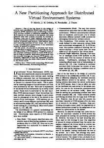
doall i = 1, N, 1 doall j = i+1, i+N, 1 doall k = i+j, 2*i+j+N, 1 LOOP BODY end doall end doall end doall
i3
1
(a)
2
3
4
i1
5
6
7
8
9
10 1
4
8
12
16
20
i2
(b) Figure 3: A motivating example
where, tjk = `jk +
Pj−1
p>k `jp tpk ,
for k + 1 ≤ j ≤ n.
S=0 From above, we observe that conditions given by the system of equations in 10 are satisfied. The augmented matrix is given by:
A formal description of detection and transformation of invariant iterators in non-uniform iteration spaces is given in Procedure 1.
1 [A|b] = 1 0
Procedure 1 Detection of an Invariant Iterator and the corresponding Transformation Matrix Input : An N-dimensional non-uniform iteration space Γ. Output : An invariant iterator.
1 1 0
The solution of Equation 14 is x = [1]. The transformation matrix thus obtained is given by:
/* Check for the existence of an invariant iterator */ for each iterator ik , for 1 ≤ k ≤ n do if Equations in 10 hold then if Equation 14 has a consistent solution then Compute the transformation matrix T Compute LT , UT , ST For each i ∈ I in each array occurrence substitute I by TI end if end if end for
1 T= 1 0 The transformed 1 LT = 0 −2
0 1 1
0 0 1
matrices LT , UT , ST are given by: 0 0 1 0 0 1 0 UT = 0 1 0 0 1 −3 0 1 ST = 0
Example 1. Consider the loop nest shown in Figure 3(a) and its corresponding iteration space in Figure 3(b). For clarity purposes, only the index points along the edges of the polytope representing the iteration space are shown. The iteration space has a parallelepiped (non-rectangular) geometry in the i-j and i-k planes. Since neither i, j nor k satisfy Equations 4 and 5, therefore, none of the iterators is invariant. Next, we find a unimodular transformation matrix for the given loop nest. Due to space limitations, we restrict the computation of the transformation matrix for the iterator j. The matrices L, U, S for the loop nest shown in Figure 3(a) are given as follows: 1 0 0 1 0 0 L = −1 1 0 U = −1 1 0 −1 −1 1 −2 −1 1
doall i = 1, N, 1 doall j = 1, N, 1 doall k = 2*i, 3*i+N, 1 LOOP BODY end doall end doall end doall
Figure 4: Unimodular transformation of the loop nest shown in Figure 3 The transformed loop nest is shown in Figure 4. In Figure 4, the iterator j is invariant. Thus, the iteration space can now be partitioned uniformly along the axis corresponding to the iterator j. As stated earlier, we partition along the
125
Procedure 2 Linearization-based Uniform Partitioning of an Iteration Space
outermost loop in order to maximize parallelism. Therefore, the second loop is moved to the outermost position before partitioning into different sets. The sets thus obtained are mapped onto different processors.
5.3
Input : A set of invariant iterators ik , for 1 ≤ k ≤ m, and the transformed loop nest LT . Output : Uniformly partitioned iteration space.
Multiple Invariant Iterators
In the previous section we derived the necessary and sufficient conditions for determining an invariant iterator and presented a unimodular loop transformation to generate the corresponding iterator. However, there may exist multiple invariant iterators in an iteration space. We employ the same approach to determine all the independent invariant iterators and their corresponding transformation matrices. However, as shown in [8], sequential application of the transformation matrices does not yield invariant iterators. To solve this problem, we employ Boyle’s mapping function [8] to determine a unified transformation matrix, derived from the independent unimodular transformation matrices.
6.
/* Iteration Reordering */ for each ik do Move ik to the outermost position end for Let lbk and ubk represent the lower and upper bound of iterator ik respectively.4 Let µk = ubk − lbk + 1, where 1 ≤ k ≤ m.
5
j ← 1; p ← P; G ← ∅ while j 6= m ∨ p 6= 1 do if gcd(µj , p) 6= 1 then p ← p/gcd(µj , p) G ← G ∪ {µj } end if j ←j+1 end while
LINEARIZATION
So far, we presented techniques to transform an iteration space to make it amenable for uniform partitioning, i.e., partitioning the outermost loop equally amongst the different processors to achieve perfect load balance. However, if the span, i.e., the difference between the upper bound and lower bound plus one, of the outermost loop is not an integral multiple of the number of processors, then uniform partitioning is not feasible. To address this, we present a linearizationbased approach to facilitate uniform partitioning. Procedure 2 presents our approach. Procedure 2 attempts to find a minimal subset of invariant iterators such that their combined span is an integral multiple of the number of processors available. If such a subset exists, then it linearizes those iterators and moves the new iterator thus obtained to the outermost position. The outermost loop is then partitioned equally amongst the different processors. For example, consider the following loop nest shown in Figure 5, where the invariant iterators have already been moved to the outermost position.
if p = 1 then Linearize the iterators corresponding to all the µs in G Move the new iterator to the outermost position Partition the outermost loop uniformly amongst P processors Exit end if /* Uniform partitioning of the iteration space along the axis corresponding to the outermost loop is not feasible */ Partition the outermost loop “equally” amongst P processors
doall i = 1, 12 doall j = 1, 8 doall k = 1, N doall l = 1, k LOOP BODY end doall end doall end doall end doall
where gcd(a, b) stands for the greatest common divisor of a and b.
can achieve perfect load balance by partitioning the iteration space amongst 12 processors, however, it will result in under utilization of the processors. As a result, it may lead to overbearing loss in parallelism, thus adversely affecting performance.6 To address the above problem, we linearize the two outermost loops as their combined span (= 12 × 8 = 96) is an integral number of the number of processors. In a similar fashion, Procedure 2 searches for a set of loops in the transformed loop nest LT such that the product of their trip counts (denoted by µ in Procedure 2) is an integral multiple of the number of processors. If there exists such a set of loops, then the corresponding loops are linearized and the loop thus obtained is partitioned uniformly amongst the P processors to yield perfect load balance. Alternatively, the
Figure 5: A sample example Let us consider the partitioning of the iteration space of the loop nest amongst 16 processors. We observe that the iterator i is invariant. However, partitioning the iteration space along the axis corresponding to i does not yield perfect load balance across all the 16 processors. Though one 4 Note that, lbk and ubk are obtained after applying transformation(s), thus they differ from the original bounds. 5 Note that, µk = constant, for 1 ≤ k ≤ m.
6
Note that using a larger number of processors does not necessarily improve the performance of the resulting partition, as discussed in [12].
126
i2
i3
do i1 = 1, N , 1 do i2 = 1, i1 + 1 , i 1 do i3 = 1, N , 1 LOOP BODY end do
end do
end do
1
(a) A loop nest
1
i1
1
i1
1
(b)
(c)
Figure 6: An illustrative example (N=6) iteration space is partitioned “equally” amongst the given processors, i.e., assuming N iterations in the outermost loop (N > P), N mod P processors are alloted dN/Pe iterations and the remaining processors are alloted bN/Pc iterations. Arguably, one could linearize L itself; however, remapping of the index expressions in the presence of affine loop bounds and strides introduces significant overhead, unlike linearization of invariant iterators.
7.
Procedure 3 Weight-based Partitioning of N-dimensional Non-Rectangular Non-Uniform Iteration Spaces Input : An N-dimensional non-uniform iteration space, Γ and P processors. Output : An optimal partitioning of the iteration space.
WEIGHT-BASED PARTITIONING
/* Compute the partial weight W (x) of Γ */
In this section we present an algorithm for partitioning an iteration space Γ across P processors, assuming that there do not exist any invariant iterators. In Procedure 3, we first compute a partial weight of the convex polytope as a function of the outermost index variable. It is important to note that the volume of a polytope provides an inaccurate estimate of the number of index points as the density of the iteration space may be nonconstant, i.e., when the induction variables have variable strides. Therefore, we follow a weight-based approach for estimating the number of index points in a polytope. Next, we compute the total weight of the convex polytope corresponding to the loop nest L using Equation 15. Then we determine the breakpoints along the i1 -axis for partitioning Γ across the given processors. The solution of Equation 16 corresponds to the k-th breakpoint, denoted by γk . Note that W (x) is a monotonically increasing function of x. Therefore, there exists only one real solution of Equation 16. In contrast, the algebraic approaches [3, 4, 8] proposed in the past for iteration space partitioning are inapplicable in such cases, as they are incapable of handling variable densities; furthermore, these previous approaches achieve load balance, even for uniform iteration spaces, by merging noncontiguous sets, thereby possibly affecting locality adversely. The breakpoints γk define the boundaries of the elementary sets in Γ. The sets thus obtained are contiguous which eliminates the need for multiple loops, required in case of non-contiguous sets. Furthermore, contiguous sets facilitate exploitation of data locality. Obviously, the same approach is applicable for determining the various sets of a partition even when the density is constant. In contrast, previous approaches [3, 4] achieve load balance across different processors at the expense of data locality, as the sets obtained by applying these approaches are non-contiguous.
x
Z
W (x) =
Z
u2
ρ1 di1
Z
un
ρ2 di2 . . .
1
ρn din
`2
`n
/* Compute the total weight W of Γ */
W =
Z
N
Z
u2
ρ1 di1 1
un
Z ρ2 di2 . . .
`2
ρn din
(15)
`n
/* Determine the kth breakpoint, γk */ W (γk ) =
k ×W P
(16)
/* Determine the loop bounds */ lbk = dγk−1 e
(17)
ubk = bγk c
(18)
where, lb and ub are the lower and upper bounds of an elementary set.
127
Next, we determine the lower and upper bounds of the loops corresponding to each set using equations 17 and 18 respectively. The algorithm is formally presented as Procedure 3 on page . Let us examine our algorithm behavior with the help of an example.
Algorithm 1 Partitioning N-dimensional Iteration Spaces with Variable Densities
Example 2. Consider the loop nest shown in Figure 6(a). The projection of the corresponding iteration space on i1 -i2 and i1 -i3 planes is shown in Figures 6(b) and 6(c) respectively. First, we compute a partial weight of the convex polytope as a function of the outermost index variable. Next, we compute the total weight of the convex polytope corresponding to the iteration space Γ. The partial and total weights are given by: Z N Z x Z i1 +1 1 dj dk W (x) = di i1 1 1 1
if InvariantIteratorExists then Partition Γ uniformly across P processors using Procedure 2 else Partition Γ using Procedure 3 end if
N
Z
numbers up to a given number N . The algorithm first “unmarks” all the integers from 2 to N . The first unmarked integer, 2, is the first prime. Then, it marks every multiple of this prime. Subsequently, it repeatedly takes the next unmarked integer as the next prime and marks every multiple of that prime. Figure 7 a) shows the kernel of TSoE. The corresponding iteration space is shown in Figure 7 b). Let us consider partitioning of the iteration space amongst 2 processors. The matrices L, U, S for the loop nest shown in Figure 7 a) are given as follows : " # " # " # 1 0 1 0 0 0 −1 1 0 1 2 1
(N − 1)(x − 1)
=
W =
Input : An N-dimensional iteration space Γ and P processors. Output : Partitioned iteration space.
i1 +1
Z di
1
1
1 dj i1
Z
N
dk = 25 1
Next, assuming 3 processors, we determine the breakpoints for the iteration space. (γ1 − 1)(N − 1) = (γ2 − 1)(N − 1) =
1 W 3 2 W 3
⇒ γ1 = 2.67 ⇒ γ2 = 4.33
First, we check the existence of an invariant iterator. For the first iterator, i.e., loop index i, we note that equations given in (10) are not applicable. The augmented matrix of the first iterator is given by: 1 1 A= 1 0 0 −2
The new loop bounds of the sets thus obtained are given by: (lb1 , ub1 )
= (1, 2), (lb2 , ub2 ) = (3, 4) (lb3 , ub3 ) = (5, 6)
From the above, we note that the system of equations represented by A is inconsistent as α 6= 0 (see the third row of A). Therefore, the first iterator is not invariant. Similarly, we observe that the second iterator is also not invariant as it does not satisfy the equations given in (10). Therefore, we employ our geometric approach, described in Section 7, for partitioning the iteration space shown in Figure 7 b). First, we determine a partial weight of the convex polytope corresponding to the iteration space of Figure 7 b).
So far, we have only considered perfect loop nests. However, our algorithm can be applied to multiway loop nests7 in a similar fashion. Detailed discussion of the above is outside the scope of this paper.
8.
THE ALGORITHM
In this section we present a unified algorithm for iteration space (with variable densities) partitioning. In Algorithm 1, the function InvariantIteratorExists determines if there exists an invariant iterator(s) in Γ using Procedure 1. If an invariant iterator(s) exists then we partition Γ uniformly along an axis corresponding to the outermost loop using Procedure 2. If an invariant iterator does not exist, then we employ a weight-based partitioning approach, as discussed in Section 7, for partitioning Γ.
9.
Z
W (x) =
x
N
Z di
3
2i dj i
2 3 x − 8982 3 Next, we determine the total weight of the convex polytope using Equation 15. 1000x2 −
=
CASE STUDY
As a case study to illustrate our algorithm, we consider The Sieve of Eratosthenes (TSoE). TSoE identifies all prime
W
N
Z =
A loop is multiway nested if there are two or more loops at the same level[14]. Note that the loops may be nested themselves.
N
Z
N
Z
i
0
2i(N − i)di
2i dj =
di 3
7
0
3
= 993172.67 Next, we determine the breakpoint for the partition.
128
j N
S1: doall i = 3, 22, 2 doall j = i, N, 2*i LOOP BODY end doall end doall S2: doall i = 22, N’, 2 doall j = i, N, 2*i LOOP BODY end doall end doall
doall i = 3, N’, 2 doall j = i, N, 2*i LOOP BODY end doall end doall
a) N’
3
i
c)
b) √ 0 Figure 7: A non-uniform iteration space. (N = 1000, N = d N e)
1000γ12 −
into nodes with several goals : vector computation within a node, loop tiling for data reuse and parallelism between tiles. In [4], Sakellariou discusses the necessary condition for partitioning a loop nest across different processors with equal workload. Based on whether the iterations are distributed among processors before or during run-time, loop partitioning can be classified as static or dynamic. In static partitioning, each processor is assigned a fixed number of iterations such that the distribution among processors is as even as possible. The most common approaches for static partitioning are:
1 2 3 γ1 − 8982 = 993172.67 3 2 ⇒ γ1 ≈ 22.655
The new loop bounds of the sets thus obtained are given by : (lb1 , ub1 ) = (3, 22), (lb2 , ub2 ) = (23, 32) Loops S1 and S2 in Figure 7 c) correspond to the two sets of the partitioned iteration space.
10.
❐ Cyclic partitioning (CP) : It distributes the iterations in a round robin fashion; thus given n iterations and p processors, processor i executes iterations i + kp, k = 0, 1, . . . , n/p. However, this approach may deteriorate performance due to false sharing.8
PREVIOUS WORK
It has been shown that loops without dependences among their iterations (traditionally known as DOALLs [5]) account for greatest amount of parallelism in numerical and scientific applications [15]. In addition, several compiler techniques [16] have been proposed to convert loops with interiteration dependences to DOALL loops for parallel execution. However, once this is done, the problem is how to partition the iteration space of the DOALLs across a given number of processors so as to minimize execution time and optimize processor utilization. In [17], Anik et al. discuss several models for parallel execution of nested loops. The simplest model is to execute the outermost loop in parallel and all the inner parallel loops sequentially. Another model involves collapsing [18] the nested loops into a single loop using compiler transformations. In another model, the inner loops are executed in parallel and a blocking barrier is used at the end of each parallel loop, which prevents the overlapping between execution of inner loops. Similarly, loop interchanging [16, 19] may be used to switch parallel loops to the outer position when the original outer loop is not parallel. However, in case of a nest of DOALLs, loop interchange is redundant w.r.t. parallel execution of the loop nest. Techniques such as loop concurrentization [20] partition the set of iterations of a loop and assigns a different subset to each processor. Irigoin and Triolet’s supernode partitioning approach [21] divides an iteration space of a loop nest
❐ Block partitioning (BP) [22] : This approach maps contiguous iterations onto processors in a consecutive manner; thus a processor i executes iterations in/p + 1 through (i+1)n/p. The efficiency of BP is governed by the block size. Assuming zero scheduling overhead, the optimal block size is k = dn/pe number of iterations. ❐ Balanced chunk scheduling (BCS) [23] : BCS attempts to distribute the total number of iterations of the loop body among processors as evenly as possible as opposed to cyclic and block partitioning which distribute only the iterations of the outer loop. An example of the latter is shown in Appendix B of [4]. However, Haghighat and Polychronopolous restrict their discussion to double loops. ❐ Canonical loop partitioning (CLP) [4] : Sakellariou introduce a notion of canonical loop nest for loop partitioning. CLP assumes that the outermost loop can be equi-partitioned into 2pm−1 parts, where p is the 8 False sharing occurs when multiple processors access data in the same cache line and one of the accesses is a ‘write’, thus causing the cache line to be exchanged between processors even though the processors access different parts of it.
129
number of processors and m is the depth of a loop nest. However, this may generate empty sets which leads to load imbalance. Moreover, CLP generates a fragmented partition i.e. each individual set is a collection of non-contiguous subsets. CLP employs an enumeration-based approach to determine the total number of index points in an iteration space. It relies on loop normalization in the presence of non-unit strides. However the introduction of floors and ceilings renders this approach nonviable in practice (see Section 7). Furthermore, determination of the set boundaries in CLP is very cumbersome. Several other techniques have been proposed in [24, 25, 26] for mapping affine loops on to multiple processors. However, these techniques focus primarily on communication minimization between the processors.
11.
CONCLUSIONS
In this paper we presented an algorithm for partitioning N-dimensional iteration spaces with variable densities. First, we presented a mathematical formulation for detecting invariant iterators in a loop nest with non-constant strides. Assuming an invariant iterator exists, we presented an approach to partition the iteration space to achieve perfect load balance. Otherwise, unlike previous approaches [3, 4], we follow a geometric approach for partitioning an iteration space. The partition thus obtained consists of contiguous sets, which facilitates exploitation of data locality. As future work, we would like to extend our approach to partition iteration spaces at run-time.
12.
ACKNOWLEDGMENTS
The first author would like to thank Siddharth Choudhuri and Mohit Singh for their valueable feedback.
13.
REFERENCES
[1] C. Polychronopoulos, D. J. Kuck, and D. A. Padua. Execution of parallel loops on parallel processor systems. In Proceedings of the 1986 International Conference on Parallel Processing, pages 519–527, August 1986. [2] E. H. D’Hollander. Partitioning and labeling of loops by unimodular transformations. IEEE Transactions on Parallel and Distributed Systems, 3(4):465–476, 1992. [3] M. R. Haghighat and Constantine D. Polychronopoulos. Symbolic analysis for parallelizing compilers. ACM Transactions on Programming Languages and Systems, 18(4):477–518, July 1996. [4] R. Sakellariou. On the Quest for Perfect Load Balance in Loop-Based Parallel Computations. PhD thesis, Department of Computer Science, University of Manchester, October 1996. [5] S. Lundstrom and G. Barnes. A controllable MIMD architectures. In Proceedings of the 1980 International Conference on Parallel Processing, St. Charles, IL, August 1980. [6] J. Foley, A. van Dam, S. Feiner, and J. Hughes. Computer Graphics: Principles and Practice. Addison-Wesley, 2nd edition in C edition, 1990.
130
[7] P. Anninos. Computational cosmology: From the early universe to the large scale structure. In Living Reviews in Relativity 4, 2001. [8] M. O’Boyle and G. A. Hedayat. Load balancing of parallel affine loops by unimodular transformations. Technical Report UMCS-92-1-1, Department of Computer Science, University of Manchester, January 1992. [9] M. Haghighat and C. Polychronopoulos. Symbolic analysis: A basis for parallelization, optimization, and scheduling of programs. In Proceedings of the Sixth Workshop on Languages and Compilers for Parallel Computing, Portland, OR, August 1993. [10] U. Banerjee. A theory of loop permutations. In D. Gelernter, A. Nicolau, and D. Padua, editors, Languages and Compilers for Parallel Computing. The MIT Press, 1990. [11] U. Banerjee. Loop Transformation for Restructuring Compilers. Kluwer Academic Publishers, Boston, MA, 1993. [12] A. Kejariwal, P. D’Alberto, A. Nicolau, and C. D. Polychronopoulos. A geometric approach for partitioning N-dimensional non-rectangular iteration spaces. In Proceedings of the 17th International Workshop on Languages and Compilers for Parallel Computing, West Lafayette, IN, 2004. [13] C. D. Meyer. Matrix Analysis and Applied Linear Algebra. SIAM, Philadelphia, PA, 2000. [14] C. Polychronopoulos. Loop coalescing: A compiler transformation for parallel machines. In S. Sahni, editor, Proceedings of the 1987 International Conference on Parallel Processing. Pennsylvania State University Press, August 1987. [15] D. Kuck et al. The effects of program restructuring, algorithm change and architecture choice on program performance. In Proceedings of the 1984 International Conference on Parallel Processing, August 1984. [16] M. J. Wolfe. Optimizing Supercompilers for Supercomputers. The MIT Press, Cambridge, MA, 1989. [17] Sadun Anik and Wen mei W. Hwu. Executing nested parallel loops on shared-memory multiprocessors. In Proceedings of the 1992 International Conference on Parallel Processing, pages III:241–244, Boca Raton, Florida, August 1992. [18] M. J. Wolfe. High Performance Compilers for Parallel Computing. Addison-Wesley, Redwood City, CA, 1996. [19] M. J. Wolfe. Advanced loop interchanging. In Proceedings of the 1986 International Conference on Parallel Processing, St. Charles, IL, August 1986. [20] D. A. Padua and M. J. Wolfe. Advanced compiler optimizations for supercomputers. Communications of the ACM, 29(12):1184–1201, December 1986. [21] F. Irigoin and R. Triolet. Supernode partitioning. In Proceedings of the Fifteenth Annual ACM Symposium on the Principles of Programming Languages, San Diego, CA, January 1988. [22] C. P. Kruskal and A. Weiss. Allocating independent subtasks on parallel processors. IEEE Transactions on Software Engineering, 11(10):1001–1016, 1985. [23] M. Haghighat and C. Polychronopoulos. Symbolic
program analysis and optimization for parallelizing compilers. In Proceedings of the Fifth Workshop on Languages and Compilers for Parallel Computing, New Haven, CT, August 1992. [24] N. Koziris, G. Papakonstantinou, and P. Tsanakas. Mapping nested loops onto distributed memory multiprocessors. In International Conference on Parallel and Distributed Systems, pages 35–43, December 1997.
[25] M. Dion and Y. Robert. Mapping affine loop nests: new results. In HPCN Europe 1995, pages 184–189, 1995. [26] M. Dion and Y. Robert. Mapping affine loop nests. Parallel Computing, 22(10):1373–1397, 1996.
131