constraints, start-up cost, and spinning reserve and is defined as .... start-up cost of the th unit; .... Application of HPSO is a new approach in solving the UC.
IEEE TRANSACTIONS ON POWER SYSTEMS, VOL. 21, NO. 1, FEBRUARY 2006
411
A Novel Approach for Unit Commitment Problem via an Effective Hybrid Particle Swarm Optimization T. O. Ting, Student Member, IEEE, M. V. C. Rao, and C. K. Loo, Member, IEEE
Abstract—This paper presents a new approach via hybrid particle swarm optimization (HPSO) scheme to solve the unit commitment (UC) problem. HPSO proposed in this paper is a blend of binary particle swarm optimization (BPSO) and real coded particle swarm optimization (RCPSO). The UC problem is handled by BPSO, while RCPSO solves the economic load dispatch problem. Both algorithms are run simultaneously, adjusting their solutions in search of a better solution. Problem formulation of the UC takes into consideration the minimum up and down time constraints, start-up cost, and spinning reserve and is defined as the minimization of the total objective function while satisfying all the associated constraints. Problem formulation, representation, and the simulation results for a ten generator-scheduling problem are presented. Results clearly show that HPSO is very competent in solving the UC problem in comparison to other existing methods. Index Terms—Hybrid particle swarm optimization (HPSO), industrial power system, optimization methods, power generation dispatch.
I. INTRODUCTION
U
NIT commitment (UC) in a power system involves determining a start-up and shut-down schedule of units to meet the required demand, over a short-term period [1]. In solving the UC problem, generally two basic decisions are involved, namely, the “unit commitment” decision and the “economic dispatch” decision. The “unit commitment” decision involves the determination of the generating units to be running during each hour of the planning horizon, considering system capacity requirements, including the reserve, and the constraints on the start-up and shut-down of units. The “economic dispatch” decision involves the allocation of the system demand and spinning reserve capacity among the operating units during each specific hour of operation. The UC problem has commonly been formulated as a nonlinear, large scale, mixed-integer combinatorial optimization problem with constraints. The exact solution to the problem can be obtained only by complete enumeration, often at the cost of a prohibitively large computation time requirement for realistic power systems [1]. Research endeavours, therefore, have been focused on efficient, near-optimal solutions. Manuscript received June 24, 2003; revised March 10, 2004. Paper no. TPWRS-00367-2003. T. O. Ting is with the Department of Electrical Engineering, Hong Kong Polytechnic University, Kowloon, Hong Kong. M. V. C. Rao and C. K. Loo are with the Faculty of Engineering and Technology, Multimedia University, 75450 Malacca, Malaysia (e-mail: zhaoen@ ieee.org). Digital Object Identifier 10.1109/TPWRS.2005.860907
UC algorithms can be applied to large-scale power systems and have reasonable storage and computation time requirements. A survey of literature on UC methods reveals that various numerical optimization techniques have been employed to address the UC problems. Specifically, there are priority list methods [2], [3], integer programming [4], [5], dynamic programming [6]–[11], mixed-integer programming [12], branch-and-bound methods [13], and Lagrangian relaxation methods [14], [15]. Among these methods, the priority list method is simple and fast, but the quality of final solution is not guaranteed. Dynamic programming methods, which are based on priority lists, are flexible but are computationally expensive. Branch-and-bound adopts a linear function to represent the fuel consumption and time-dependent start cost and obtains the required lower and upper bounds. The disadvantage of the branch-and-bound method is the exponential growth in the execution time with the size of the UC problem. The integer and mixed-integer methods adopt linear programming technique to solve and check for an integer solution. These methods have only been applied to small UC problems and have required major assumptions that limit the solution space. The Lagrangian relaxation method provides a fast solution, but it may suffer from numerical convergence and solution quality problems. Aside from the above methods, there is another class of numerical techniques applied to the UC problem. Specifically, they are artificial neural networks [16], [17], simulated annealing (SA) [18], and genetic algorithms (GAs) [19]–[22]. These methods can accommodate more complicated constraints and are claimed to have better solution quality. SA is a powerful, general-purpose stochastic optimization technique, which can theoretically converge asymptotically to a global optimum solution with probability 1. One main drawback, however, of SA is that it takes a large CPU time to find the near-global minimum. GAs are a general-purpose stochastic and parallel search methods based on the mechanics of natural selection and natural genetics. It is a search method and has the potential of obtaining a near-global minimum. In this paper, we apply the hybrid particle swarm optimization (HPSO) method in solving the UC problem. A description of the HPSO method is presented in Section II. Then a detailed explanation of HPSO approach is given in Section III. The UC problem formulation is given in Section IV, while Section V explains the constraints satisfaction techniques employed in this experiment. Numerical tests and results using HPSO is presented in Section VI. Finally, a conclusion is given in Section VII.
0885-8950/$20.00 © 2006 IEEE
412
IEEE TRANSACTIONS ON POWER SYSTEMS, VOL. 21, NO. 1, FEBRUARY 2006
II. PARTICLE SWARM OPTIMIZATION PSO was introduced by Kennedy and Eberhart in 1995 [23] as an alternative to GAs. The PSO technique has ever since turned out to be a competitor in the field of numerical optimization. Similar to GA, a PSO consists of a population refining its knowledge of the given search space. PSO is inspired by particles moving around in the search space. The individuals in a PSO thus have their own positions and velocities. These individuals are denoted as particles. Traditionally, PSO has no crossover between individuals, has no mutation, and particles are never substituted by other individuals during the run. Instead, the PSO refines its search by attracting the particles to positions with good solutions. Each particle remembers its own best position found so far in the exploration. This position is called personal in (1). Additionally, among these best and is denoted by , there is only one particle that has the best fitness, called the global best and is denoted by in (1). The velocity of the th dimension is defined as
(1) where is known as the inertia weight as described in [24] and [25]. The best found position for the given particle is denoted by , whereas is the best position known for all particles. and are set to constant values, which are The parameters 1.2 and 2.8 (Section VI explains why these values are chosen), is a randomly generated value berespectively, whereas tween 0 and 1. As mentioned, the subscript denotes the th dimension of a particle. The position of each particle is updated on every iteration. This is done by adding the velocity vector to the position vector, as described in (2) It has been noticed that members of the group seem to share information among them, a fact that leads to increased cohesion or efficiency (e.g., in search of food) of the group. Some scientists suggest that knowledge is optimized by social interaction and thinking is not private but also interpersonal. Therefore, particle swarms have not only individual but also a collective intelligence, simply by virtue of their social interactions. The simplest version of PSO lets every individual move from a given point to a new one that is a weighted combination of the individual’s best position ever found and of the individual’s best . The choice of the PSO algorithm’s parameters position, (such as the inertia weight) seems to be of utmost importance for the speed and efficiency of the algorithm. III. HPSO APPROACH TO UC The original version of PSO [23] operates on real values. The term “hybrid particle swarm optimization” was first mentioned in [40], whereby the term hybrid meant the combination of PSO and GA. However, in our approach here, hybrid is meant to highlight the concept of blending real valued PSO [solving economic load dispatch (ELD)] with binary valued PSO (solving
UC) running independently and simultaneously. The binary PSO (BPSO) is made possible with a simple modification to the particle swarm algorithm. This BPSO solves binary problems similar to those traditionally optimized by GAs. Kennedy and Eberhart [26] showed that the binary particle swarm was able to successfully optimize the De Jong [27] suite of test functions. Further, Kennedy and Spears [28] compared the binary particle swarm algorithm to GAs comprising crossover only, mutation only, and both crossover and mutation, in Spears’ multimodal random problem generator. It was seen that the particle swarm found global optima faster than any of the three kinds of GAs in all conditions except for problems featuring low dimensionality. In our simulation results to solve the ELD, we proved that this is true as the results show better convergence for PSO and in the feasible environment. In binary particle swarm, can take on values of 0 or 1 only. The velocity will determine a probability threshold. If is higher, the individual is more likely to choose 1, and lower values favor the 0 choice. Such a threshold needs to stay in the range [0.0, 1.0]. One straightforward function for accomplishing this is common in neural networks. The function is called the sigmoid function and is defined as follows: (3) The function squashes its input into the requisite range and has properties that make it agreeable to be used as a probability threshold. A random number (drawn from a uniform distribution is set to 1 between 0.0 and 1.0) is then generated, whereby if the random number is less than the value from the sigmoid function as illustrated in the following: If
then
else
(4)
In the UC problem, represents the on or off state of generator . In order to ensure that there is always some chance of a bit flipping (on and off of generators), a constant can be set at value rethe start of a trial to limit the range of . A large sults in a low frequency of changing state of generator, whereas a small value increases the frequency of on/off of a generator. is often set at , so that there is always at In practice, least a good chance that a bit will change state. This is to limit so that does not approach too close to 0.0 or 1.0. In this functions similarly to the mutation rate in binary model, GAs. IV. UC PROBLEM FORMULATION In this section, we first formulate the UC problem and then present a detailed PSO algorithm for solving the UC problem. The objective of the UC problem is the minimization of the total production costs over the scheduling horizon. Therefore, the objective function is expressed as the sum of fuel and start-up costs of the generating units. For generators, the operation cost is defined mathematically as shown in the following: TPC
ST
(5)
TING et al.: NOVEL APPROACH FOR UC PROBLEM VIA AN EFFECTIVE HPSO
The operating cost accumulates over the total number of operating hours , where = 24, which represents 24 h of operation for each unit of generator. Therefore, (5) is rewritten as TPC
ST
(6)
In (5), TPC is the total production cost for units of generators, whereas TPC in (6) denotes the total production cost for units of generators over number of operating hours. Owing to the operational requirements, the minimization of the objective function is subjected to the following constraints: 1) Power balance constraint
413
V. CONSTRAINTS SATISFACTION Recently, several methods for handling infeasible solutions for continuous numerical optimization problems have emerged [29]–[32]. Some of them are based on penalty functions. They differ, however, in how the penalty function is designed and applied to infeasible solutions. They commonly use the cost function to evaluate a feasible solution, i.e., (13) and the constraint violation measure straints are usually defined as
for the
con-
(14) (7) or 2) Spinning reserve constraint (15) (8) 3) Generation limit constraint (9) 4) Minimum up-time constraint (10)
where = max . In other words, is the magnitude of the violation of the th inequality constraint, where . Similarly, is the violation magnitude of the th . This means is the equality constraint, where number of inequality constraints, whereas is the number of equality constraints. Then the total evaluation of an individual , which can be interpreted as the error (for a minimization problem) of an individual , is obtained as
5) Minimum down-time constraint
(16) (11)
where the notations used are as follows: TPC total production cost of the power generation; fuel cost function of the th unit with generation at the th hour. Usually, it is a quadratic output polynomial with coefficients and as follows: (12)
ST
MU MD
number of generators; number of hours; generation output of the th unit at the th hour; start-up cost of the th unit; on/off status of the th unit at the th hour and when off, when on; load demand at the th hour (set to 10% of ); spinning reserve at the th hour; minimum generation limit of the th unit; maximum generation limit of the th unit; minimum up-time of the th unit; minimum down-time of the th unit; duration during which the th unit is continuously on; duration during which the th unit is continuously off.
where is a penalty parameter of a positive or negative constant for the minimization or maximization problem, respectively. By associating a penalty with all constraint violations, a constrained problem is transformed to an unconstrained problem such that we can deal with candidates that violate the constraints to generate potential solutions without considering the constraints. A. Satisfying Power Demand and Reserve Constraints With respect to the theoretical explanation above, we formulate the objective of the UC problem as a combination of total production cost as the main objective with power balance and spinning reserve as inequality constraints, whereby TPC (5), and is equivalent to the blend of power balance and spinning reserve constraints. Consequently, the formulation of the objective function is as shown below: (17) TPC (18) As discussed, is the penalty factor that is computed at the th generation defined by . The choice of determines the accuracy and speed of convergence. From the
414
IEEE TRANSACTIONS ON POWER SYSTEMS, VOL. 21, NO. 1, FEBRUARY 2006
experiment, a greater value of increases its speed and convergence rate. Due to this reason, a value of 100 for is selected. The pressure on the infeasible solution can be increased with the number of generations, as discussed in the Kuhn–Tucker optimality theorem, and penalty function theorem provides guideis set to 1 if a vilines to choose the penalty term. In (18), olation to constraint (7) occurs and C1 = 0 whenever (7) is not is also set to 1 whenever a violation of violated. Likewise, (8) is detected, and it remains 0 otherwise. The second term in is 10% of the penalty factor is the reserve constraint, where . Thus, (18) can also be written as power demand
Once the total power generated is greater than the demand, minus the error from the current generator in order to exactly meet the demand. Check the range, if exceed
or less than
re-initialize randomly within power limits of a generator. Next Else if total power For
Demand then
MaxUnit to 1 step -1
Set generator with lowest priority to operate at minimum capacity accordingly. Once the total power generated is less then the demand, add the error to the current
TPC
generator in order to exactly meet the demand. Check the range, if exceed
or less than
re-initialize randomly within power limits of a
(19)
generator. Next End if
By substituting (5) into (19)
Loop
B. Satisfying the Generation Limit Constraints
ST
(20) Equation (20) is the fitness function for evaluating every particle in the population of PSO for an hour. For hours, (20) is redefined as in (21), shown at the bottom of the page. To decrease the pressure of constraint violation error on the , a set of major feasible solutions that satfitness function isfy the power demand is generated before evaluation of (21) is considered. Based on the current research [33]–[37], feasible solutions satisfying the power demand and reserve constraints are considered prior to ED. This assures that the PSO explores in a feasible environment, which reduces the computation time as well as improves the quality of the solution. The pseudocode below illustrates the process whereby the feasible power values are generated based on its demand. MaxUnit in the pseudocode is the maximum number of generators. Do while Demand is not met If total power generated < Demand then For
The initial values of power are generated randomly within power limits of a generator. As particles explore the searching space, starting from initial values, which are generated randomly within the power limit as derived in (9), they do encounter cases whereby the power generated exceeds the boundary (minimum or maximum capacity) and therefore violate the constraint in (9). To avoid the boundary violation, we reinitialize the value whenever it is greater than the maximum capacity or smaller than the minimum capacity of a generator. Again, the reinitialization is done within the power limits of a generator. C. Satisfying the Minimum Up and Down Time Constraints The technique used to satisfy the min-up (MU) and min-down (MD) time in this paper is extremely simple. As the solution is based upon the best particle ( ) in the history of the entire population, constraints are taken care of by forcing the binary to change its state whenever either MU or value in MD constraint is violated. However, this may change the current fitness, which is evaluated using (21). It implies that the might no longer be the best among all the other current particles. To correct this error, the will be revaluated using the same equation. Ramping can be incorporated by adding the ramping cost into the total production cost TPC (5) of this paper, similar to [43, (1)]. Thereby, (5) can be redefined as
to MaxUnit
Set generator with top priority to operate at
TPC
maximum capacity accordingly.
ST RU
RD
ST (21)
TING et al.: NOVEL APPROACH FOR UC PROBLEM VIA AN EFFECTIVE HPSO
where RU and RD are the ramp-up and ramp-down costs for the th generator. Another method that can be considered is proposed in [44]. This is successfully implemented by combining and of the generators as dethe ramping rate into the picted in [44, (5)]. Both [43] and [44], however, do not consider any MU and MD constraints.
415
TABLE I PARAMETER SENSITIVITY ANALYSIS FOR UC (50 RUNS)
VI. NUMERICAL SIMULATIONS The PSO program was implemented in Visual Basic language and the simulation was carried out on a ten-generator system; the data is given in Tables III and IV. The setting for HPSO is as follows: - Population Size ; - Maximum Iterations ; - Dimension Number of generators, MaxUnit ; - Maximum Velocity ; - Inertia Weight . The population size of 20 is generated on an hourly basis. This means that each hour will have 20 independent particles. Each particle consists of a MaxUnit dimension, where MaxUnit is the maximum number of generators available (regardless of on or off status). This means each dimension of a particle represents a generator. Each hour will have its own independent particle. Hence, the total cost is the summation of hourly-based costs. Before proceeding to the simulation, careful selection of parameter settings is important to produce a competent result. The parameter sensitivity analysis is presented in Table I. This analysis features the constant inertia weight set from 0.1 to 1.0 with increment of 0.1. The decreasing [24] from 0.9 to 0.4 is also tested. The range from 0.9 to 0.4 for linearly decreasing performs best in [40] and [41]. However, this method does not perform well in the UC problem. This gives us an idea that the settings of PSO are actually problem dependent. The different is tested with a set of and , whereby following the sugges. The analysis of these three parameters tion in [42], , and are found in (1). Based on the results, and and are chosen for another 100 runs, as HPSO seems to perform the best with these settings. The simulation result of HPSO is shown in Table II, with Fig. 1 showing the best solution of UC and power generation. The result does not show any violation of reserve and power demand constraints, except for hour 23, whereby the error is so small that it can just be ignored. This is because feasible solutions that satisfy both these constraints are generated before evaluating fitness of every particle in PSO. By observing the generated power as in Fig. 1, we can conclude that the generated , as power for each hour is equivalent to the power demand depicted in Table IV. One major advantage of HPSO is its simplicity of the algorithm as compared to any other techniques in existence so far. HPSO is much faster than other techniques, such as the GA approach. From the result in Table II, the best total cost obtained is $563 942.3. This is certainly a better solution than the solution obtained using GAs, having a total cost
TABLE II COMPARISON OF RESULTS
of $565 825, as reported in [22] and [38]. The same cost is obtained using the DP approach [22]. DP is a sort of deterministic method in solving the UC problem. The DP method is capable of finding the global optimal solution, and the method has been utilized as a benchmark method recently, even if it takes a long time to find the global optimal solution. However, DP for UC [22] cannot generate a global optimal solution due to time-dependent constraints that are MU and MD, as specified in (10) and (11) in Section IV. Since this method is a deterministic method, the solutions obtained have the same value for different runs. This is the reason for unavailable values under “Average” and “Worst” in Table II. Likewise, the same reason applies for LR [22] and LRGA [38] methods. As mentioned, the best cost encountered by HPSO out of 100 runs is $563 942.3, whereas the worst cost is $565 785.3. The average for this 100 runs is $564 772.3. From the comparison, it is obvious that the HPSO method is superior to other methods, such as GAs, evolutionary programming (EP), and GA based on unit characteristic classification (UCC-GA) in [37]. In comparing the worst solution obtained by HPSO (565 785.3), UCC-GA is better in the worst value obtained, 565 606. It means that the quantity of “randomness” in HPSO is greater than UCC-GA. This could be a possibility that leads HPSO to a better solution. One major advantage of HPSO is the conceptual simplicity of the algorithm, resulting in a cheaper computational cost and faster speed of convergence. However, it is not easy to determine its parameter settings for optimal performance of a particular problem, as it is quite time consuming. The literature does provide some useful thumb rules to get started on any problem that has been found to work well.
416
IEEE TRANSACTIONS ON POWER SYSTEMS, VOL. 21, NO. 1, FEBRUARY 2006
TABLE III GENERATOR SYSTEM OPERATOR DATA
Fig. 1.
Best solution of UC and power generation total cost = $563 942:3.
TABLE IV LOAD DEMANDS FOR 24 h
VII. CONCLUSION Application of HPSO is a new approach in solving the UC problem. Results demonstrate that HPSO is a very competent
method to solve the UC problem. HPSO generates better solutions than the other methods, mainly because of its intrinsic nature of updates of positions and velocities. The second reason is due to the hourly basis solution. This is somehow similar to the “divide and conquer” strategy of solving a problem. Owning to this hourly solution, the complexity of the search is greatly reduced. The total objective function is the sum of objectives and constraints, which are fuel cost, start-up cost, spinning reserve, and power demand. For a better soluunit of generators are constantly tion, generated powers by checked so that feasible particles that meet the power demand are always met. This reduces the pressure of the constraint violation of the total objective function. The MU and MD times are treated separately by forcing the generator to turn on or off in order to fulfill this constraint. The result obtained from the simulation is most encouraging in comparison to the best known solution so far.
TING et al.: NOVEL APPROACH FOR UC PROBLEM VIA AN EFFECTIVE HPSO
APPENDIX A. Power Demand Satisfaction for Economic Dispatch
REFERENCES [1] A. J. Wood and B. Wollenberg, Power Generation Operation and Control, 2nd ed. New York: Wiley, 1996. [2] R. M. Burns and C. A. Gibson, “Optimization of priority lists for a unit commitment program,” in Proc. IEEE/Power Engineering Society Summer Meeting, Paper A 75 453-1, 1975. [3] G. B. Sheble, “Solution of the unit commitment problem by the method of unit periods,” IEEE Trans. Power Syst., vol. 5, no. 1, pp. 257–260, Feb. 1990. [4] T. S. Dillon, K. W. Edwin, H. D. Kochs, and R. J. Taud, “Integer programming approach to the problem of optimal unit commitment with probabilistic reserve determination,” IEEE Trans. Power App. Syst., vol. PAS-97, no. 6, pp. 2154–2166, Dec. 1978.
417
[5] L. L. Garver, “Power generation scheduling by integer programming development of theory,” IEEE Trans. Power App. Syst., vol. PAS-18, pp. 730–735, Feb. 1963. [6] W. L. Snyder Jr., H. D. Powell Jr., and J. C. Rayburn, “Dynamic programming approach to unit commitment,” IEEE Trans. Power App. Syst., vol. PAS-2, pp. 339–350, May 1987. [7] P. G. Lowery, “Generation unit commitment by dynamic programming,” IEEE Trans. Power App. Syst., vol. PAS-102, pp. 1218–1225, 1983. [8] C. K. Pang and H. C. Chen, “Optimal short-term thermal unit commitment,” IEEE Trans. Power App. Syst., vol. PAS-95, no. 4, pp. 1336–1346, Aug. 1976. [9] C. K. Pang, G. B. Sheble, and F. Albuyeh, “Evaluation of dynamic programming based methods and multiple area representation for thermal unit commitment,” IEEE Trans. Power App. Syst., vol. PAS-100, no. 3, pp. 1212–1218, May 1981. [10] C. C. Su and Y. Y. Hsu, “Fuzzy dynamic programming: An application to unit commitment,” IEEE Trans. Power Syst., vol. 6, no. 3, pp. 1231–1237, Aug. 1991. [11] Z. Ouyang and S. M. Shahidehpour, “An intelligent dynamic programming for unit commitment application,” IEEE Trans. Power Syst., vol. 6, no. 3, pp. 1203–1209, Aug. 1991. [12] J. A. Muckstadt and R. C. Wilson, “An application of mixed-integer programming duality to scheduling thermal generating systems,” IEEE Trans. Power App. Syst., pp. 1968–1978, 1968. [13] A. I. Cohen and M. Yoshimura, “A branch-and-bound algorithm for unit commitment,” IEEE Trans. Power App. Syst., vol. PAS-102, no. 2, pp. 444–451, 1983. [14] A. Merlin and P. Sandrin, “A new method for unit commitment at Electricite de France,” IEEE Trans. Power App. Syst., vol. PAS-102, pp. 1218–1255, May 1983. [15] F. Zhuang and F. D. Galiana, “Toward a more rigorous and practical unit commitment by Lagrangian relaxation,” IEEE Trans. Power Syst., vol. 3, no. 2, pp. 763–770, May 1988. [16] Z. Ouyang and S. M. Shahidehpour, “A hybrid artificial neural network/dynamic programming approach to unit commitment,” IEEE Trans. Power Syst., vol. 7, no. 1, pp. 236–242, Feb. 1992. [17] H. Sasaki, M. Watabable, J. Kubokawa, N. Yorino, and R. Yokoyama, “A solution method of unit commitment by artificial neural networks,” IEEE Trans. Power Syst., vol. 7, no. 1, pp. 974–985, Feb. 1992. [18] F. Zhuang and F. D. Galiana, “Unit commitment by simulated annealing,” IEEE Trans. Power Syst., vol. 5, no. 1, pp. 311–317, Feb. 1990. [19] D. Dasgupta and D. R. McGregor, “Thermal unit commitment using genetic algorithms,” Proc. Inst. Elect. Eng., Gener., Transm., Distrib., vol. 141, no. 5, pp. 459–465, Sep. 1994. [20] C. L. Huang, J. S. Tzeng, P. C. Yang, and H. T. Yang, “Implementation of genetic algorithm for unit commitment,” in Proc. 14th Symp. Electrical Power Engineering, Taiwan, R.O.C., 1993, pp. 439–446. [21] G. B. Sheble and T. Maifeld, “Unit commitment by genetic algorithm and expert system,” Elect. Power Syst. Res., vol. 30, pp. 115–121, 1994. [22] S. A. Kazarlis, A. G. Bakirtzis, and V. Petridis, “A genetic algorithm solution to the unit commitment problem,” IEEE Trans. Power Syst., vol. 11, no. 1, pp. 83–92, Feb. 1996. [23] J. Kennedy and R. Eberhart. Particle swarm optimization. presented at Proc. IEEE Int. Conf. Neural Networks. [Online]. Available: http://www.engr.iupui.edu/~shi/Conference/psopap4.html. [24] Y. H. Shi and R. C. Eberhart, “A modified particle swarm optimizer,” in Proc. IEEE Int. Conf. Evolutionary Computation, Anchorage, AK, May 4–9, 1998. [25] Y. H. Shi and R. C. Eberhart, “Empirical study of particle swarm optimization,” in Proc. Congr. Evolutionary Computation, Washington, DC, Jul. 6–9, 1999. [26] J. Kennedy and R. C. Eberhart, “A discrete binary version of the particle swarm algorithm,” in Proc. Int. Conf. Systems, Man, Cybernetics. Piscataway, NJ, 1997, pp. 4104–4109. [27] K. A. De Jong, “An analysis of the behavior of a class of genetic adaptive systems,” Ph.D. dissertation, Univ. of Michigan, 1975. [28] J. Kennedy and W. M. Spears, “Matching algorithms to problems: An experimental test of the particle swarm and some genetic algorithms on the multimodal problem generator,” in Proc. Int. Conf. Evolutionary Computation. Piscataway, NJ, 1998, pp. 78–83. [29] Z. Michalewicz and N. Attia, “Evolutionary optimization of constrained problems,” in Proc. 3rd Annu. Conf. Evolutionary Programming, A. V. Sebald and L. J. Fogel, Eds. River Edge, NJ: World Scientific, 1994, pp. 98–108. [30] A. S. Homaifar, H. Y. Lai, and X. Qi, “Constrained optimization via genetic algorithms,” Simulation, vol. 62, pp. 242–254, 1994.
418
[31] D. Powell and M. Skolnick, “Using genetic algorithm in engineering design optimization with nonlinear constraints,” in Proc. 5th Int. Conf. Genetic Algorithms, S. Forrest, Ed. Los Altos, CA: Morgan Kaufmann, 1991, pp. 151–157. [32] M. Schoenauer and S. Xanthakis, “Constrained GA optimization,” in Proc. 5th Int. Conf. Genetic Algorithms, S. Forrest, Ed. Los Altos, CA: Morgan Kaufmann, 1993, pp. 573–580. [33] K. S. Swarup and S. Yamashiro, “Unit commitment solution methodology using genetic algorithm,” IEEE Trans. Power Syst., vol. 17, no. 1, pp. 87–91, Feb. 2002. [34] J. M. Arroyo and A. J. Conejo, “A parallel repair genetic algorithm to solve the unit commitment problem,” IEEE Trans. Power Syst., vol. 17, no. 4, pp. 1216–1224, Nov. 2002. [35] T. Senjyu, H. Yamashiro, K. Shimabukuro, K. Uezato, and T. Funabashi, “A fast solution technique for large scale unit commitment problem using genetic algorithm,” in Proc. IEEE/Power Engineering Society Asia Pacific Transmission Distribution Conf. Exhib., vol. 3, 2002. [36] T. Senjyu, K. Shimabukuro, K. Uezato, and T. Funabashi, “A fast technique for unit commitment problem by extended priority list,” IEEE Trans. Power Syst., vol. 18, no. 2, pp. 882–888, May 2003. , “A unit commitment problem by using genetic algorithm based [37] on unit characteristic classification,” in Proc. IEEE Power Engineering Society Winter Meeting, vol. 1, 2002, pp. 58–63. [38] C. P. Cheng, C. W. Liu, and C. C. Liu, “Unit commitment by Lagrangian relaxation and genetic algorithms,” IEEE Trans. Power Syst., vol. 15, no. 2, pp. 707–714, May 2000. [39] K. A. Juste, H. Kita, E. Tanaka, and J. Hasegawa, “An evolutionary programming to the unit commitment problem,” IEEE Trans. Power Syst., vol. 14, no. 4, pp. 1452–1459, Nov. 1999. [40] S. Naka, T. Genji, T. Yura, and Y. Fukuyama, “A hybrid particle swarm optimization for distribution state estimation,” IEEE Trans. Power Syst., vol. 18, no. 1, pp. 60–68, Feb. 2003. [41] H. Yoshida, K. Kawata, Y. Fukuyama, S. Takayama, and Y. Nakanishi, “A particle swarm optimization for reactive power and voltage control considering voltage security assessment,” IEEE Trans. Power Syst., vol. 15, no. 4, pp. 1232–1239, Nov. 2000. [42] M. Clerc and J. Kennedy, “The particle swarm: Explosion stability and convergence in a multi-dimensional complex space,” IEEE Trans. Evol. Comput., vol. 6, no. 1, pp. 58–73, Feb. 2002. [43] C. Wang and S. M. Shahidehpour, “Optimal generation scheduling with ramping costs,” IEEE Trans. Power Syst., vol. 10, no. 1, pp. 60–67, Feb. 1995.
IEEE TRANSACTIONS ON POWER SYSTEMS, VOL. 21, NO. 1, FEBRUARY 2006
[44] G. Baskar, N. Kumarappan, and M. R. Mohan, “Optimal dispatch using improved �-based genetic algorithm suitable for utility system,” Elect. Power Compon. Syst., vol. 31, pp. 627–638, 2003.
T. O. Ting (S’03) was born in 1978. He received the B.S. degree from University Sarawak Malaysia, Sarawak, Malaysia, in 2002 and the M.E. degree from Multimedia University, Malacca, Malaysia, in 2004. He is currently working toward the Ph.D. degree from the Department of Electrical Engineering, Hong Kong Polytechnic University, Kowloon, Hong Kong. He is a Tutor with Multimedia University. His current research interests are optimization techniques, evolutionary computation, and power system.
M. V. C. Rao was born in 1941. He received the B.S. degree in 1962 from Sri Venkateswara University, Tirupati, India, the M.E. degree in 1965 from Madras University, Madras, India, and the Ph.D. degree in 1973 from the Indian Institute of Technology-Madras. He is currently a Professor with Multimedia University, Malacca, Malaysia. His field of research work is control system theory. His research interests are in the areas of discrete data systems, nonlinear programming methods, generalized predictive control, fuzzy logic control, neural networks, and evolutionary computation.
C. K. Loo (M’02) received the B.E. degree (with first-class honors) in mechanical engineering from the University of Malaya, Kuala Lumpur, Malaysia, in 1996 and the Ph.D. degree from the University of Science Malaysia, Pulau Pinang, Malaysia. He has been with the Faculty of Engineering and Technology, Multimedia University, Malacca, Malaysia, since 2001. His fields of interest are soft computing, fault diagnosis intelligent robotic control, and quantum image processing.