A Novel Available Bandwidth Estimation and Tracking Algorithm Albert Cabellos-Aparicio1, Francisco J. Garcia2, Jordi Domingo-Pascual1 Department of Computer Architecture, Technical University of Catalonia, Barcelona, Spain 2 Agilent Laboratories Scotland, Agilent Technologies, Edinburgh EH30 97G, UK {acabello,jordid}@ac.upc.edu,
[email protected] 1
Abstract— The available bandwidth (AB) of an end-to-end path is its remaining capacity and it is an important metric for several applications. That´s why several available bandwidth estimation tools have been published recently. Most of these tools use the Probe Rate Model. This model is based on the concept of selfinduced congestion and requires that the tools send a packet train at a rate matching the available bandwidth. The main issue with this model is that these tools congest the path under study. In this paper we present a novel available bandwidth estimation tool that takes into account this issue. Our tool is based on a mathematical model that sends packet trains at a rate lower than the AB. The main drawback of this model is that it is not able to track the AB. To solve this issue we propose to apply Kalman Filters (KF) to the model. By applying these filters we can produce real-time estimations of the available bandwidth and monitor its changes. In addition the KFs are able to filter the noisy (erroneous) measurements improving the overall accuracy. We also present an extensive evaluation of our tool in different network scenarios and we compare its performance with that of pathChirp (a state-of-the-art available bandwidth estimation tool). Keywords:Available Bandwidth, Measurement, Kalman Filter
I.
INTRODUCTION
The Available Bandwidth (AB) of an end-to-end path is its remaining capacity, that is, the amount of traffic that can be sent along the path without congesting it. Recently, the area of end-to-end AB estimation has attracted considerable interest. Basically because the AB is an important metric for several applications such as overlay networks, dynamic server selection, and inter-domain path monitoring. As a result, several estimation techniques and tools based on active measurements have been developed. Most of the proposed tools designed to estimate the AB fall into two categories: the Probe Rate Model (PRM) and the Probe Gap Model (PGM). The first model uses packet trains and it is based on the concept of self-induced congestion. Informally, if one sends a packet train at a rate lower than the AB along the path, then the arrival rate of the packet train at the receiver will match the rate at the sender. However if the sending rate is greater or equal than the AB then the packet train will congest the queues along the path and the receiving rate will be lower than the sending rate. Tools such as Delphy [1], TOPP [2], PathLoad [3], IGI/PTR [4], pathChirp [5],
BART [7] and AB [9] use this model. The second model (PGM) uses packet pairs and bases its estimation on the differences of input and output time gaps of the packet pairs [6]. However C. Dovrolis et al. showed that this model can underestimate the AB of multi-hops paths with one-hop persistent traffic [20]. The PRM model has been used in many AB estimation tool and it has been shown as very accurate. However it suffers from one basic problem. PRM-based tools must send probe traffic at a rate equal or greater than the AB in order to estimate it. This will fill the queues along the path congesting it. This means that, for each estimation, a PRM-based tool will congest the measured path during a certain period of time. In fact, A.Shriram et al. showed recently in [16] that tools such as PathLoad [3] can significantly impact the responses time of TCP connections. In this paper we present a novel AB estimation tool that takes into account this issue. Our main objective is to estimate the AB without sending probe traffic at a rate equal or greater than the actual AB, thus reducing considerably the impact on the measured path. Our tool is intended for network administrators that aim to track, and obtain long-term statistics of the usage (AB) of a path without severely impacting its performance. The tool is based on the mathematical model presented in Forecaster [8]. This model shows that there is a linear relation between the utilization of a path and the probe traffic rate sent. Forecaster estimates this straight line by sending two packet trains at different rates (always below the AB). Then it “projects” the line and estimates the AB. Although Forecaster shows that this model is very accurate it requires sending two separated packet trains in order to estimate the AB. This packet trains may be sent at a very low rate (i.e Capacity/10). During this interval Forecaster assumes that the AB does not change. However this does not hold on a real path and may lead Forecaster to incorrect estimates. In addition, this issue makes it very difficult for Forecaster to efficiently track the AB under sudden variations. As we will see, our tool is able to produce an estimation per packet train. One aspect of our tool is that it does not send packet trains at a higher rate than the AB. Another aspect is that it produces an estimation per packet train. This means that our tool reduces
the impact on the queues along the path and that it is able to track the AB. This is achieved by exploiting the above mentioned linear model. However instead of “projecting” the line or using linear regression, we rely on Kalman Filtering [11]. The Kalman Filters (KF) are an efficient recursive filter that estimates the state of a linear system from a series of noisy measurements. With KFs we are able to produce an estimation per measurement (instead of one estimation for two measurements) and filter noisy (erroneous) measurements. This means that KFs allows us to create a continuous monitoring tool able to track the AB and improve the overall accuracy. The remainder of this paper is organized as follows. First we discuss the related work, and then we present the design of our available bandwidth estimation tool. Next we show the evaluation of our tool and finally we present the conclusions. II.
RELATED WORK
The area of available bandwidth estimation has attracted much attention recently and many tools have been published. As it has been shown in the previous section, most of these tools use either the Probe Rate Model or the Probe Gap Model. In this section we will present only the tools related to our approach. S.Ekelin et al. presented in [7] BART, a PRM-based AB estimation tool that exploits Kalman Filters. BART uses a linear model that relates the interpacket strain (the time gap between two consecutives packets) with the probe traffic rate. Then the AB is computed as the point where the line intercepts the horizontal axis. In fact BART’s model is similar to ours, the main difference is that their linear model is defined above the AB while ours is defined below the AB. That´s why BART has to congest the tight link in order to produce an estimation. Finally, at the best of the authors’ knowledge, the only AB estimation tool that does not send probe traffic matching the AB is Forecaster [8]. The tool presented here is based on this mathematical model but produces estimations using KFs instead of projecting a line. In addition our tool is able to track the dynamic variations in the AB. III.
ABEST DESIGN
In this section we present the design of our tool. First we present the mathematical model, next we discuss how we apply Kalman Filters to the model and then we discuss how the utilization is estimated. Finally we show the algorithm used to track the AB. A. Mathematical Model The utilization of a queue in a single-hop scenario is: (1) Where is the probability that the queue is void. Most of the existing AB measurement techniques rely on using a constant-rate fluid cross-traffic model. This means that these techniques assume that the cross-traffic has infinitely small packet size and arrives at the hop at a constant rate. In fact, X. Liu et al. showed in [19] that the tools that use a constant-rate fluid model can underestimate the AB under certain conditions.
However eq. 1 does not make any assumptions about the nature of the cross-traffic. If we transmit probe traffic at a rate the utilization can be expressed as:
through this link, then (2)
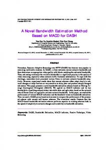
Where is the capacity of link . For the multi-hop case, K. Harfoush et al. showed in [8] a first order approximation of eq. 2 for a multi-hop scenario: (3) Where and are constants. This equation states that there is a linear relation between the utilization of a path and the rate of the probe traffic sent. Figure 1 shows that, as the probe traffic rate increases so does the utilization (linearly). At a certain rate the utilization will reach 1 (the path is fully loaded) then, the available bandwidth of the path is .
r2
r1
slope = a
Vertical Intercept = b
AB Figure 1. The tool’s linear model.
This means that with this model we can estimate the AB without sending the probe traffic at the AB rate. Once the linear equation (eq. 3) has been estimated the AB can be computed as the point where the straight line reaches 1 (i.e utilization = 1): (4) B. The Kalman Filters Our tool uses Kalman filtering to estimate the linear equation (eq. 3). The KFs are able to estimate a system defined by a state vector , affected by an input through noisy measurements. In our case the network is our system and the noisy measurements are the estimations of the utilization. The system is also affected by a noise and the measurements have a noise . Then, the system is governed by the linear stochastic difference equation: (5)
With a measurement
Thus, the following equation governs our system:
that is:
(8)
(6) Where the subscript refers to the discrete time and relates the state of the previous time step with the state of the new time step . Similarly, relates the control input to the state while relates the state with the measurement. Then, the KF estimates the process by using a form of feedback control: the filter estimates the process state at some time and then obtains feedback in the form of (noisy) measurements. The KF algorithm has two steps, in the first step (“time update”) the filter projects forward in time the state of the system and obtains an a priori estimate. In the second step (“measurement update”) the filter uses a new measurement to correct the a priori estimate to produce an improved a posteriori estimate. After each time and measurement update pair, the process is repeated with the previous a posteriori estimates used to project or predict the new a priori estimates. This recursive nature is one of the main advantages of the Kalman Filters. The KFs assume that the system is linear and that the system noise and the measurement noise are Gaussian and independent. Please refer to [11] for further details on Kalman Filters.
The measurements are governed by equation (6). We define as: (9) This way the measurements (eq. 6) are seen by the KF as the actual utilization of the system under our probe-traffic load. Finally, the predictor equations defined by the KFs in our particular case are: (10) (11) And the corrector equations are: (12) (13) (14)
Figure 2. Mean absolute error of the estimation of the utilization using different distributions.
In our case the state vector that describes the system represents our linear model (the parameters of the sloping straight line from eq. 3): (7) As it has been shown in [8] our system is linear. We drop the input (and consequently because in our particular case the network is affected by the intensity of our probe traffic and the cross-traffic. As we cannot estimate the intensity of the cross-traffic we do not use this particular parameter. It is important to remark that, as we will show later, this does not affect the accuracy of the results. In addition we drop ( because the state of the previous time step of the network will be the same than the state of the new time step.
Where the “minus” superscript refers to the a priori estimates (before the measurement correction). is the estimate of the error covariance matrix, its value will be updated by the KF each time step. is the Kalman gain, a very important parameter of the KFs. This gain is computed (in each time step) in eq. 12 and weights the new measurement with the a priori estimate in eq. 13. Finally and represent the process and measurement noise covariance respectively. These are key parameters in the KFs. The authors in [7] suggest computing as the variance of the estimations of the utilization. However this does not represent accurately the measurement noise because, at the end, our goal is to measure the AB. That´s why we compute as the variance of the estimations of the AB. As our results show this improves the overall accuracy of our tool and helps it to track the actual AB. Regarding , the process noise covariance is a 2x2 matrix that represents the variability of the system. This value must be set manually and is a key parameter when considering the behavior of the KF. A high means that the KFs will consider the prediction as less accurate while the measurements will be considered as very accurate. Therefore the KFs will set the Kalman gain accordingly and each new measurement will be weighted heavier. Low values for mean the opposite. We will come back to this in the result’s section. C. Estimating Utilization As we have seen, at this point if we can estimate the utilization of a link we can estimate the AB through eq 4. In this subsection we discuss how to design an optimal estimator for the utilization. Eq. 1 defines the utilization as the probability that there is at least one packet in the queues of the path. In order to estimate the utilization of a path the authors in [8] suggest sending a packet train, end to end, and compute the fraction of
packets that have experienced queuing delay along the path. Probe packets are time stamped at the sender and at the receiver. Then the minimum one-way delay of the set of packets is computed. This minimum delay corresponds to the delay suffered by a packet that has not encountered queuing delay. Therefore, the fraction of packets with a greater delay than the minimum delay is the fraction of packets that suffered queuing delay. Let be the set of one-way delays suffered by the packets of the packet train. Then the utilization is estimated as: (15) According to the PASTA [13] property, if this packet train is sent with exponential inter-departure times, the packets arriving in the queuing system will sample the system queues, on average, as an outside observer would at an arbitrary point in time. However F. Baccelli et al showed in [14] that Poisson probes are not unique in their ability to sample without bias. That is why we have evaluated other distributions in order to analyze which distribution samples the queues better for our particular estimator. We tested a range of different distributions by sending 104 packet trains (of 200 packets and 1500B as packet size) at different rates on a single link fed with Poisson packet arrivals. The link is simulated using ns2 and the crosstraffic packet sizes are distributed as in the Internet (see [15] for details): 50% (40 bytes), 10% (576 bytes) and 40% (1500 bytes). Z. Zhang et al. showed in [21] that the Internet traffic has weak correlation over time scales less than 100ms and stronger correlations at time scales greater than 1s. The duration of our packet trains is around 100ms, this means that a Poisson cross-traffic model suffices. The packet trains are sent with different inter-departure time distributions: Periodic, Poisson, Uniform [0.9µ,1.1µ], Uniform [0,2µ] and Pareto (shape parameter α=1.16). The experiment is performed with different link loads (utilization={0,0.3,0.6,0.75,0.9}). For each packet train we have computed the absolute error when estimating the utilization.
As Figure 2 (in the previous page) shows the distribution that minimizes the error when estimating the utilization is the Poisson distribution while the worst one are the Periodic and Uniform [0.9µ,1.1µ] distributions. In fact, the exponentially distributed packet trains are not severely impacted by the load of the link and the mean error is always below 0.07. The Periodic and Uniform [0.9µ,1.1µ] distributions create “constant” packet trains where the inter-departure time of the packets is very similar. The behavior of these packet trains is roughly described by the Probe Rate Model. If the rate of the packet train is above the AB then almost all the packets are queued, and thus the utilization is overestimated. If the rate is below the AB then the packets do not congest the tight link queue and thus the utilization is underestimated. Regarding the Pareto and Uniform [0,2µ] distributions figure 2 shows that they are more accurate under high link loads that under low link loads. This is because these distributions have also some periodicity. When the link load is at 90% the cross-traffic rate congests the tight link queue and almost all the packets are queued. This means that the utilization for this very special case is accurately estimated. At this point we have evaluated different distributions for estimating the utilization and concluded that the optimal one is the Poisson distribution, where the inter-departure time of the packets belonging to a packet train are exponentially distributed. However we still need to evaluate which is the optimal packet train length and which is the optimal packet size. We have performed the same experiment than before but using different packet train lengths and different packet sizes. Figure 3 (note that the X-Axis uses a log-scale for clarity) shows the mean absolute error for different packet train lengths under different link loads. As the figure shows packet trains with a length lower or equal to 150 packets suffer from a large error when estimating the utilization.
Figure 4. Mean absolute error using different packet sizes.
Figure 3. Mean absolute error using different packet train lengths.
Regarding packet trains longer than 150 packets the mean error is bounded to 0.06. In addition, the error is not significantly impacted by the utilization of the link under study. In fact the error is slightly reduced as the packet train length increases. However it is important to remark that long packet
trains suffer from one basic problem, the utilization may change during the transmission of the packet train and this may lead to incorrect estimates. Thus, there is a tradeoff between the accuracy of the estimations and the duration of the measurement. We believe that the optimal length for our packet trains is 200 packets. Longer packet trains (250,300,350…) have slightly less error, however as the figure shows this extra accuracy is not justified since the duration of the measurement is increased dramatically (i.e packet trains of 250 packets last 25% more than packet trains of 200 packets). Finally, regarding the packet sizes figure 4 shows the mean error when estimating the utilization using different packet sizes (40B,100B,500B,1000B and 1500B). As the figure shows the optimal packet size is 1500B (this result agrees with the conclusions reached in [10]). As the figure shows when we use packet sizes of 40 and 100 bytes the mean error is larger (up to 0.08) than when we use packet sizes of 500, 1000 and 1500 bytes. In fact, these packet sizes have a very similar error, where the maximum mean difference is 5.5 10-3. We chose 1500 bytes as the packet size for our packet trains because we need to send less packets for each packet train, in addition these packets will have larger inter-departure times. This will make the implementation of our tool easier, specially when dealing with the “Interrupt Coalescence” [18] issue.
Our tool sends probe traffic at a random rate (uniformly distributed [0,MAX_RATE] and estimates the utilization. Then it uses the KFs to estimate the parameters of the linear model ( and ) and finally it produces an estimation of the AB using eq. 4. The algorithm can be easily implemented. It does not require time synchronization because it estimates the utilization by comparing the OWD of the packets (note that the actual value of the OWD it is not needed). It does not require the accurate computation of the dispersion of the packets. Therefore it may not suffer from the “Interrput Coalescence” issue described in [18]. Since KFs are recursive, it does not require storing past values. The main drawback (and advantage) of the algorithm is that some parameters need to be set, evaluated and tuned.
As a summary figure 5 shows the expected performance of our packet trains (exponentially distributed, 200 packets and 1500 bytes as packet size). The figure shows that in 90% of the cases the error is bounded to 0.08 and that the tool’s packet trains provide a good performance. The figure also shows that under high link loads (>90%) the accuracy of our packet trains is slightly impacted. We will come back to this later. Figure 6. The algorithm used to estimate the AB
IV.
EVALUATION
This section presents the evaluation of our tool. First we detail the methodology that we have used and then we present the results of the evaluation.
Figure 5. CDF of the expected performance of our packet trains
D. The AB Estimation and Tracking Algorithm Figure 6 details the algorithm used by this tool to estimate the AB. The algorithm uses the following initial parameters: MAX_RATE which is an upper bound for the rate of the probe traffic and INTERVAL which is the measurement interval, x which represents the initial guess of the AB and Q, which is the covariance matrix of the process noise.
A. Methodology We have evaluated our tool through extensive simulations. We have implemented it in NS2 and used a wide range of scenarios to analyze its accuracy and show its limitations. We have used four different scenarios with different number of links and different capacities. Our scenarios aim to represent the actual configuration of a backbone path, thus we simulate very high-speed links (up to 10Gbps). Usually these high-speed links are in the middle of the path, just like in a real Internet backbone path. For each scenario we have run two different sets of experiments. In the first set we load the different scenarios with static cross-traffic rate. That is, the AB does not change during the experiments. The different links are loaded with non hoppersistent cross-traffic, this means that it interacts with our probe traffic on one link. With this set of experiments we aim to evaluate the accuracy of the tool under different loads. In the second set we load the different scenarios with variable crosstraffic rate. In this case the cross-traffic is hop-persistent and
TABLE I.
SCENARIOS USED TO EVALUATE OUR TOOL. FOR EACH SCENARIO WE SHOW THE CAPACITY OF THE LINKS AND THE LOAD OF EACH LINK. THE RIGHTMOST COLUMN SHOWS THE ACTUAL AB.
Scenario I
Static
100 Mbps 0.0 0.3 0.95
Variable
Scenario II
Static
1000 Mbps 0.0 0.2 0.9
Variable
Scenario III
Static
51 Mbps 0.0 0.5 0.1
Variable
Scenario IV
Static
1000 Mbps 0.0 0.2 0.95
Variable
we aim to evaluate if the tool is able to accurately track the AB. It is important to remark that this is our main objective. Regarding the cross traffic we use the same configuration than for the previous experiments (sec. III). The distribution for the packet sizes are as measured in the Internet: 50% (40 bytes), 10% (576 bytes) and 40% (1500 bytes) and the cross-traffic model is Poisson.
622 Mbps 10 Mbps 0.0 0.0 0.4 0.2 0.2 0.01 AB varies: 4, 8, 6, 10 Mbps 10000Mbps 100 Mbps 0.0 0.0 0.1 0.5 0.1 0.7 AB varies: 80, 40, 60, 100 Mbps 4976 Mbps 100 Mbps 0.0 0.0 0.1 0.2 0.2 0.7 AB varies: 21, 51, 41, 31 Mbps 4976 Mbps 622 Mbps 100 Mbps 0.0 0.0 0.0 0.1 0.1 0.3 0.1 0.1 0.1 AB varies: 80, 100, 40, 60 Mbps
Available Bandwidth
10 Mbps 8 Mbps 5 Mbps
100 Mbps 50 Mbps 30 Mbps
51 Mbps 25 Mbps 30 Mbps
100 Mbps 70 Mbps 50 Mbps
(case B) the path is at a half-load, this is a typical scenario. The last case (case C) is a worst-case scenario where at least one link is highly congested (up to 95%). This third case is used to evaluate the performance of the tool in an extreme situation and analyze its limitations. For the variable AB experiments we use variable cross-traffic rate. Since the tool is intended to collect long-term statistics of the AB we have simulated large variations of the AB (and thus, of the cross-traffic rate). Finally, we compare the results of our tool with that of pathChirp [5]. pathChirp is considered as one of the best [16] available bandwidth estimation tools and uses the PRM model, this means that it congests at least one link along the path in order to estimate the AB. It is important to remark that it has also been shown in [16] that among the PRM-based tools pathChirp is considered as one of the less intrusive.
Figure 7. Mean error when estimating the AB for the static cases
Table I summarizes the configuration of our experiments. For the static AB experiments we have three different cases. In the first case (case A) the path is not loaded with cross-traffic. This case is used as a best-case scenario. In the second case
B. Results On the one hand, figure 8 presents the results of the simulations for all the static scenarios (case A,B and C). All the results are presented using Interquartile Range Boxes where the box represents the middle 50% of the estimations and thus, the line in the middle of the box is the median. The upper/lower whiskers extends to the minimum/maximum data point within 1.5 box heights from the bottom/top of the box. Finally the cross represents the mean of the estimations. Each case was simulated during 300 seconds for both tools. The (red) cross highlights the actual available bandwidth for each case and for each scenario. On the other hand, figure 7 shows the mean relative error for all the different cases:
d
Figure 8. Results of the simulations for the static cases
(16) As both figures show both tools are very accurate for the case A (in all the different scenarios). In this particular case both tools show very good accuracy where the mean relative error is around 0.1. As it has been said before this is a simple case, from the figures we can also see that our tool has larger variability than pathChirp. This depends on the configuration of the covariance matrix of the process noise Q and can be tuned; we will come back to this later. However it is important to remark that this does not affect the accuracy of our tool.
upgrade a link. The main benefit of our technique is that the impact on the performance of the network is lower. Regarding the variable experiments, figure 9 shows the mean relative error for the different scenarios. In this experiment the AB has sudden variations and both tools need to rapidly adjust its estimations. As the figure shows our tool is more accurate than pathChirp, in this case the average error for pathChirp is 0.12 while for our tool is 0.06. It is important to remark that one of our objectives is to accurately track the changes of the AB and collect long-term statistics.
Regarding the second case (B), where the network is at half load, both tools also show high accuracy with a similar mean error. We believe that this is the most common case in the internet and the mean relative error for the four scenarios is 0.065 for our tool and 0.085 for pathChirp. Finally, for the third case (C) where the network is highly congested both tools show lower accuracy. Specifically the last scenario has a backbone link of 4976Mbps under a high utilization (0.95). This is considered as a worst-case scenario and it is not very common on the Internet. In this case the error of our tool is due to an incorrect estimation of the utilization. The problem is that when our tool is operating near the full utilization it is difficult for our Kalman Filters to estimate the slope of the straight line (in the mathematical model). This is because a highly congested link may drop packets, making difficult to accurately estimate the utilization. As the figure shows pathChirp’s accuracy is also affected by the same reason. We believe that this is a tradeoff because we estimate the AB without sending packet trains at the same rate than the AB. This can be solved by designing a special estimator for this very special case (when the estimated utilization is very high). This special estimator should take into account losses. In any case if our tool detects that a link is highly congested it just needs to report it, this should be enough for upper layers (such as a routing algorithm) to make a decision, or to an ISP´s to
Figure 9. Mean error when estimating the AB for the variable cases
Summarizing our tool’s accuracy is similar to that of pathChirp for the static experiments while it is better for the variable cross-traffic rate experiments. Our evaluation has also shown the main limitation of our tool in highly congested paths (the same applies to pathChirp). In addition we have seen that the covariance matrix of the process noise Q is a key parameter that can tune the behavior of our tool. This matrix represents
the uncertainty of the process. Large values of Q will help our tool react quicker to large variations of the AB, however it will also increase the variability. Low values of Q mean the opposite. In fact, this parameter may be used to tune the behavior of our tool in different scenarios. If we want to monitor the AB at short time-scales it is better to use a large Q (it will react quicker) while if we want to monitor it at large time-scales it is better a low Q (it will be more stable). In this paper we have used a large value of Q, that´s why our tool has larger variability than pathChirp but it is more accurate for the variable experiments. We have used the same value of Q along all the experiments (see figure 6). The evaluation and optimization of this parameter is left as future work.
Finally, as future work we plan to design an adaptative algorithm that chooses the optimum MAX_RATE according to the produced estimations and we plan to evaluate the Q matrix. REFERENCES [1] [2]
[3]
[4]
V.
CONCLUSIONS
The AB is one of the most important metrics in the area of network measurements. Many tools have been published and most of them use the Probe Rate Model. This models sends probe traffic at a rate similar (or even larger) than the AB. This leads to congestion and reduces the performance of the network under measurement. We have presented a novel available bandwidth estimation tool that benefits from a mathematical model that uses the utilization of the path to estimate the AB. In order to estimate the utilization this model sends packet trains at a lower rate than the AB, thus reducing the impact on the path. However, the main issue of this model is that it requires two measurements to produce an estimate. If the AB changes during these measurements the produced estimation is incorrect. Therefore it is not able to track the changes of the AB. Our proposed solution is to apply the Kalman Filters to this model. With the Kalman Filters we just need one measurement to produce an estimation. Incorrect (noisy) estimations of the utilization are filtered by the use of KFs improving the overall accuracy. In addition the KFs are able to track the changes of the AB. Our tool´s main goal is to collect long-term statistics of the variations of the AB for ISPs. We have evaluated our tool under a wide range of scenarios to evaluate its accuracy. The results show that our tool has a comparable accuracy with that of pathChirp (considered as one of the best AB estimation tools) for the static experiments. In addition we show the limitations of our tool. When the path is highly congested our tool has lower accuracy (the accuracy of pathChirp is also severely affected). We believe that this is not very common on the Internet and that it can be solved by designing an estimator of the utilization that takes into account packet losses. Regarding the scenarios where the AB varies over time (our main goal) we found that our tool accurately tracks it and shows better accuracy than pathChirp. Summarizing, the main benefit of our tool compared with others is that it does not send packet trains at a rate comparable to the AB while providing a good estimation. The main drawback is that, when operating under high congestion, the accuracy is lower.
[5]
[6]
[7] [8] [9] [10]
[11]
[12]
[13] [14] [15]
[16] [17]
[18]
[19]
[20] [21]
V. J. Ribeiro, M. Coates, R. H. Riedi, S. Sarvotham, and R. G. Baraniuk. Multifractal cross traffic estimation. In Proc. of ITC spec B. Melander, M. Bjorkman, and P. Gunningberg. A New End-to-End Probing and Analysis Method for Estimating Bandwidth Bottlenecks. In GLOBAL INTERNET SYMPOSIUM, 2000. M. Jain and C. Dovrolis. Pathload: A Measurement Tool for End-to-End Available Bandwidth. In PASSIVE AND ACTIVE MEASUREMENTS, Fort Collins, CO, March 2002. N. Hu and P. Steenkiste. Evaluation and Characterization of Available Bandwidth Techniques. IEEE JSAC Special Issue in Internet and WWW Measurement, Mapping, and Modeling, 2003. V. J. Ribeiro, R. H. Riedi, R. G. Baraniuk, J. Navratil, and L. Cottrell. pathChirp: Efficient Available Bandwidth Estimation for Network Paths. In PASSIVE AND ACTIVE MEASUREMENT Workshop, 2003. J. strauss et al, “A Measurement Study of Available Bandwidth Estimation tools”, in Proc. INTERNET MEASUREMENT CONFERENCE (IMC) 2003. Svante Ekelin et al, “Real-Time Measurement of End-to-End Available Bandwidth using Kalman Filtering”, IEEE NOMS 2006 Mradula Neiginhal et al “Measuring Bandwidth Signatures of Network Paths”, IFIP NETWORKING 2007 Yu Cheng et al “New Exploration of Packet-Pair Probing of Available Bandwidth Estimation and Traffic Characterization”, IEEE ICC 2007 C. Dovrolis et al “Packet-Dispersion Techniques and a CapacityEstimation Methodology”, IEEE/ACM Transactions On Networking, Vol. 12, No. 6, 2004 Kalman, Rudolph Emil, “A New Approach to Linear Filtering and Prediction Problems”, Transactions of the ASME--Journal of Basic Engineering, 1960 Svante Ekelin, Martin Nilsson, Erik Hartikainen, Andreas Johnsson, JanErik Mångs, Bob Melander and Mats Björkman: Real-Time Measurement of End-to-End Available Bandwidth using Kalman Filtering, IEEE NOMS 2006 R.W. Wolff, Poisson arrivals see time averages, Opns. Res., 30, pp. 223-231, 1982 F. Baccelli et al, “The Role of the PASTA property in Network Measurement”, SIGCOMM 2006. Cooperative Association for Internet Data Analyisis “NASA Ames Internet Exchange Packet Length Distributions” http://www.caida.org/analysis/AIX/plen_hist Alok Shriram and Jasleen Kaur, “Empirical Evaluation of Techniques for Measuring Available Bandwidth”, INFOCOM 2007. Erik Hartikainen and Svante Ekelin: Tuning the Temporal Characteristics of a Kalman-Filter Method for End-to-End Bandwidth Estimation, IEEE E2EMON 2006 R.Prasad and M.Jain, Effects of Interrupt Coalescence on Network Measurements, PASSIVE AND ACTIVE MEASUREMENT, April 2004. Xiliang Liu, Kaliappa Ravindran, and Dmitri Loguinov, A Stochastic Foundation of Available Bandwidth Estimation: Multi-Hop Analysis, IEEE/ACM Transactions on Networking, April 2008. C. Dovrolis et al, “The Probe Gap Model can Underestimate the Available Bandwidth of Multihop Paths” SIGCOMM 2006. Z. Zhang, V.J. Ribeiro, S.B. Moon, C. Diot, “Small-time scaling behaviors of Internet backbone traffic: an empirical study”, INFOCOM 2003