A novel framework for solving the state assignment

A novel framework for solving the state assignment problem for event-based specifications Luciano Lavagno, Cho W. Moon, Robert K. Brayton, Alberto Sangiovanni-Vincentelli Department of Electrical Engineering and Computer Sciences University of California Berkeley, CA 94720, USA Abstract We propose a novel framework to solve the state assignment problem arising from the signal transition graph (STG) representation of an asynchronous circuit. We first establish a relation between STGs and finite state machines (FSMs). Then we solve the STG state assignment problem by minimizing the number of states in the corresponding FSM and by using a critical race-free state assignment technique. State signal transitions may be added to the original STG. A lower bound on the number of signals necessary to implement the STG is given. Our technique significantly increases the STG applicability as a specification for asynchronous circuits.

1 Introduction Asynchronous circuits are playing an increasingly important role in digital designs for two main reasons: 1. Interface circuits, which are inevitably asynchronous, are becoming a bottleneck in the design process. The overall system throughput depends heavily on interface circuits, but unlike data paths or synchronous controllers they are designed mostly with little or no CAD support. As a result, interface circuits, despite their small size, can take a disproportionately large amount of design effort. 2. The clock skew problem, that is increasingly difficult to handle in today’s high-speed synchronous designs, can be completely eliminated with asynchronous designs, resulting in more modular, faster, and possibly less power-consuming designs. Despite this, CAD support for asynchronous design remains weak. The main reason is the difficulty in dealing with the hazards which cause a system to deviate from its specified behavior. In [8] and [12] techniques were proposed to produce a hazard-free implementation from a graphical specification called the Signal Transition Graph (STG)[3] under either bounded wire delay or unbounded gate delay models. The STG is based on a type of Petri net called the free-choice net, which is expressive enough for specifying concurrency, sequencing, and conflict, yet simple enough for analysis. The specification is complete in that both the system and the environment behaviors are specified. Sufficient conditions for an STG to be implementable have been given by [3]. The most restrictive condition is the Complete State Coding (CSC) property ([12]), which requires that the signals specified by the STG completely define the circuit state. Until now the burden of satisfying the CSC property has been placed mostly on the designer. [19] and [17] address this problem but only in the context of marked graphs, which are a subset of STGs. In this paper we propose a new framework to satisfy the CSC property on any live STGs by formulating the problem as the conjunction of the constrained state minimization and critical race-free state assignment problem. We first give a procedure to derive from an STG an equivalent FSM representation that completely captures the state information implicit in the STG. Minimization of this FSM allows us to prove necessary conditions on the number of state signals required to implement it. This proposed framework is general enough to embed also previous methods to solve the CSC problem for some specific sub-classes of STGs, such as [17].

1

Ri+ Ri− Ro+ Ai+ Ai− Ro−

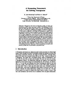
Figure 1: STG Specification of PLA Interface Circuit We also address how to extract from the minimized FSM sufficient conditions for the STG to have the CSC property. We propose to apply a critical race-free state assignment algorithm (such as the one proposed by Tracey [14]). Using the new states codes, we insert appropriate signal transitions in the STG. At this point, techniques such as [8] [12] can be used to obtain a hazard-free implementation. This paper is organized as follows. Section 2 defines the terms used in this paper and discusses some previous work. Section 3 gives an informal overview of the whole approach. Section 4 describes how STGs are translated into FSMs. Section 5 describes our state minimization process. Section 6 describes our critical race-free state assignment technique. Section 7 describes how to insert state signals in the STG so that it can be implemented. Section 8 gives some experimental results. Section 9 concludes this paper and outlines future work.

2

Preliminaries

2.1 Definitions 2.1.1

Signal Transition Graph

An STG is an interpreted free-choice Petri net introduced by Chu [3](whence most of the following definitions are drawn) for specifying asynchronous control circuits. It is a 4-tuple, hT; P; F; m0 i. T is a set of transitions described by s  f+; ?g, where s+ represents a 0 to 1 transition on signal s and s? a 1 to 0 transition. P is a set of places which can be used to specify conflict or choice. F represents the flow relation between transitions and places; namely, F  (T  P ) [ (P  T ). A marking is an assignment of nonnegative integers (denoting the number of tokens) to each place. m0 defines the initial marking or the initial state of the STG. A transition t is called the fanout transition of a place p if (p; t) 2 F . Likewise, t is called the fanin transition of p if (t; p) 2 F . Fanout places and fanin places are defined similarly. An STG is a free-choice Petri net because for each place p 2 P with multiple fanout transitions, p is the unique fanin place for all its fanout transitions. An STG is an interpreted free-choice Petri net because each t 2 T is interpreted as a physical signal change on some input or output signal. An example of an STG is shown in Fig 1. Places with only one fanin and one fanout transition are omitted, and input signal transitions are underlined. A transition is enabled if all its fanin places have at least one token. An enabled transition must eventually fire. For example, if s+ fires, the value of signal s changes from 0 to 1. After a transition fires, a token is removed from each of its fanin places and a token is added to each of its fanout places. A place with more than one fanout transition is called a free-choice (or input-choice) place if all the fanout transitions belong to input signals. The choice as to which transition will be enabled is made by the environment. A marking m0 is live if for all markings mi reachable from m0 , every transition can be enabled through some sequence of firings from mi . A net is live if its initial marking is live. A marking m0 is safe (sometimes referred to as 1-bounded) if no 2

place can ever be assigned more than one token after any sequence of firings from m0 . A net is safe if its initial marking is safe. A Marked Graph (MG) is a Petri net where each place p has exactly one fanin and one fanout transition. A State Machine (SM) is a Petri net where each transition t has exactly one fanin and one fanout place. Hack ([5]) proved that: Theorem 1 Let N be a live safe free-choice Petri net. Then 1.

N can be decomposed into strongly connected SM components that cover it (each component is sequential and exhibits non-deterministic choice).

2.

N it can be decomposed into strongly connected MG components that cover it (each component has concurrency and does not exhibit non-deterministic choice).

“Covering” means that each transition and place of the net has a correspondent in at least one SM component and a correspondent in at least one MG component, and that no component is a proper subgraph of another component. An STG is defined as live,1 if: 1. the underlying net is live and safe, and 2. for each signal t there is at least one SM component, initially marked with exactly one token, such that: (a) it contains all transitions t of t,

(b) each path from a transition t to another transition t (i.e. both rising or falling) contains also the complementary transition t . This ensures that each signal in the circuit always has a well-defined value in all markings reachable from the initial one, because a rising and falling transition for the same signal can never be concurrently enabled and each signal must have alternate rising and falling transitions. Two transitions t1 ; t2 in a live STG are concurrent if there exists a reachable marking m where both t1 and t2 are enabled, t1 is not disabled by the firing of t2 , and t2 is not disabled by the firing of t1 . 2.1.2

State Graph

The state graph (SG) is a directed graph obtained by performing a reachability analysis on the STG starting from the initial marking m0 . An SG is a 2-tuple, hV; E i, where V is a set of states and E a set of edges  V  V . A state s1 is connected to a state s2 by an edge e, if there exists a marking m2 (corresponding to state s2 ) which is reached from marking m1 (corresponding to state s1 ) by firing a single transition t. The edge e is labeled with t. In the rest of the paper we will use the term SG state to identify also the corresponding STG marking. 2.1.3

Complete State Coding

The procedures given by [3, 8, 12] to produce a circuit implementing an STG specification require that each SG state is assigned a binary label, with the values of signals specified by the STG, that is consistent with the firing transitions on the SG edges. For each s1 ! s2 labeled with transition t+ , the value of signal t in the label of s1 is 0, in the label of s2 is 1 (and vice-versa for t? ). All other signals must have the same value in both labels. Such a labeling always exists if the STG is live. The boolean function for each output signal t of the STG can then be defined as mapping the binary label of each SG state s into the implied value of t in s:



if a transition of t is enabled in state s, then the implied value for t is the complement of the value of t in the binary label of s.



otherwise the implied value for t is the value of t in the binary label of s.

A necessary and sufficient condition for the existence of an implementation of a live STG is called the Complete State Coding (CSC) property ([12]). The CSC property is satisfied if 1 Notice

the distinction between live net and live STG.

3

RiAiRo

Ai− s1 110 Ri−

Ri−

s2 100

Ai− s3 010

s4 000 Ri+

Ri+ Ai− s5 110

s6 100

Ro+

Ro+ Ai−

s7 111 Ri−

s8 101 Ri−

s9 111 Ri− Ro−

Ai+

Ai− s10 011

Ro− Ai+

s11 001

s12 011

Figure 2: State Graph with CSC violation

 

no two different states are assigned the same binary label (Unique State Coding property [16]) or when the same binary label is assigned to two different states, the transitions of the output signals enabled in the two states must be identical.

Thus, only the input transitions enabled in two states with the same binary label may be different, and it is assumed that the environment knows how to distinguish them. Figure 2 gives an example of CSC violation. States s1 and s5 are assigned the same binary label 110 but s5 has an enabled output transition Ro+ which s1 does not have. The CSC violation also occurs due to states (s2; s6), (s7; s9) and (s10; s12). 2.1.4 Finite State Machines Most of the following definitions are from [15]. A Finite State Machine (FSM) model of a sequential circuit is a six-tuple (S; X; Z; N; O; R), where:

     

S is a finite set of internal states (often called simply states) of the circuit. X is a finite set of input states of the circuit (a binary vector representing the value of its input signals). Z is a finite set of output states of the circuit (a binary vector representing the value of its output signals). N (i; s) is a relation from a present state/input state pair to the next states (i.e. N  X  S  S ). O(i; s) is a relation from a present state/input state pair to the output states (i.e. O  X  S  Z ). R  S is a set of initial (or reset) states. In this work we only consider incompletely specified deterministic FSMs, where both N (i; s) and O(i; s) are incompletely specified functions (which must be both either specified or unspecified for a given (i; s) pair), and R is a singleton set. If N (i; s1 ) = fs2 g for some i we say that s2 is a successor of s1 , and s1 is a predecessor of s2 .

Input and output signals are collectively referred to as the external signals of the circuit, and in this work they correspond exactly with the input and output signals specified by an STG from which the FSM is derived (as shown in Section 4). In the synchronous case the FSM changes state once per clock cycle. In the asynchronous case the FSM changes state every time its input state changes. An FSM can also be represented as a directed graph, where:



each vertex is associated with an internal state 4



each edge (also called a transition) is labeled with an input state/output state pair, and is directed from the present state vertex to the next state vertex.

This FSM representation, in tabular form, is called Flow Table in [15]. A stable state of an FSM is a pair i; s such that N (i; s) = fsg, i.e. a self-loop in the graph representation. An FSM is normal if every unstable state leads directly to a stable state (i.e. for every input state i, for every pair of states s; s0 such that N (i; s) = fs0 g, if s 6= s0 then N (i; s0 ) = fs0 g) A set c of states of an FSM is output compatible if s1 ; s2 2 c; O(i; s1 ) 6= ; O(i; s2 ) 6=  ) O(i; s1 ) = O(i; s2 ), i.e. for each input state i 2 X for each state s 2 c, the output label, if defined, is the same. A set c of states implies a set c0 of states if c0 = s2c fN (i; s)g. A set c of states is compatible if it is output compatible and it does not imply an output incompatible set through any sequence of implications2. A set C of compatibles of an FSM is a set of maximal compatible sets of states such that every state belongs to at least one compatible. A set C of compatibles is closed if for each input state i, for each pair of states s1 ; s2 2 c there exists a c0 2 C such that if N (i; s1 ) 6=  and N (i; s2 ) 6=  then N (i; s1 )  c0 and N (i; s2 )  c0 . A closed set  of compatibles is a closed partition of the states of the FSM if every state belongs to one and only one compatible (called block). A closed partition  is derived from a closed set of compatibles C if every block of  is a subset of a compatible of C . A state s of an FSM F covers a state s0 of another FSM F 0 if all finite sequences of input states applicable to F 0 with initial state s0 are also applicable to F with initial state s and if, for all such sequences of input states, the sequence of output states of F with initial state s is the same as that of F 0 with initial state s0 . An FSM F covers another FSM F 0 if every state in F 0 is covered by at least one state of F . Two FSMs are equivalent if they cover each other. An FSM is minimized if there exists no equivalent FSM with fewer states. FSM minimization amounts to finding a closed set of compatibles of minimum cardinality, and then creating one state of the minimized FSM for each compatible ([15], see also Section 5.3). An encoded FSM 3 is an FSM whose states have been assigned a binary label, using the value of a set of state signals. A race is a transition of an encoded FSM where more than one state signal changes. The race is critical if the behavior of the FSM depends on the outcome of the race, i.e. on which signal changes first.

S

2.1.5 Multi-valued boolean functions and decision diagrams A multi-valued boolean variable is a variable vi that can take any value from a finite set Si . A boolean function of a set of multi-valued variables fvi g is a mapping from the cartesian product of the Si into f0; 1g. The properties of ordinary boolean functions (where all the variables have Si = f0; 1g) can be directly extended to boolean functions of multi-valued variables ([10]). A multi-valued decision diagram (MDD, see [1] and [6]) is a rooted directed acyclic graph where:

  

every leaf node is labeled with either the value 1 or 0. every non-leaf node is labeled with a multi-valued boolean variable. every edge is labeled with one value of the variable corresponding to its source node.

An MDD represents a boolean function over the variables associated with the MDD labels in the following way. Every element of the domain of the function defines a unique path from the root to a leaf, by following edges labeled with the variable values associated with the domain element. The function has value 1 on all the points that correspond to paths to the leaf 1, and 0 on all the other points (they obviously corresponds to paths to 0). Conversely every path from the root to the 1 leaf defines a (possibly partial) assignment of values that makes the associated function evaluate to 1 (and similarly for 0).

2.2

Previous work

Early work in the area of Unique State Coding enforcement (for example [19] and [16]) concentrated on the introduction of constraints within an MG, using a sufficient condition as a guidance. Namely both [19] and [16] recognized that if all pairs of signals in the STG are locked using a chain of handshaking pairs, then the MG satisfies the Unique State Coding condition. We will briefly show in Section 5 how to interpret this sufficient condition within our framework, and how to use it to reduce the number of state signals. 2 Notice 3 The

that for incompletely specified FSMs the compatibility relation in not transitive, and as such it is not an equivalence relation. encoded FSM is called Flow Matrix in [15].

5

Also the synthesis methodology developed by Martin et al. ([2]), even though it starts from a different specification formalism, basically guarantees CSC (a sub-case of what they call non-interference) by handshaking, if possible, otherwise by heuristic state variable insertion ([11]). More recently Vanbekbergen et al. ([17]) proposed a technique to transform an MG so that it satisfies CSC. The technique is based on the identification of pairs of SG states that cause a CSC violation. Each pair of such states is connected by an edge in an undirected graph called the constraint graph4 . Then coloring this graph provides, according to the author, a lower bound on the number of state signals required for CSC. This approach, even though it was originally proposed only for MGs, bears some resemblance with the framework that we propose for general STGs. In fact graph coloring has been used since long ago as a heuristic for FSM minimization ([18]). Furthermore Vanbekbergen did not recognize the need to use critical race-free encoding. Critical races would show up as further violations of CSC in the encoded STG. Thus the main advantage of our framework over [17] is the recognition that CSC falls within a much more general problem, previously known as state minimization/critical race-free encoding ([15]), and that constraint graph coloring can be considered only as a heuristic technique to solve the general problem. Kishinevsky et al. ([7]) also presented a complete synthesis methodology for asynchronous circuits starting from an event-based specification, called Transition Diagrams, that is very similar to MGs. They also used graph coloring to identify regions of the state graph that must be distinguished using state signals. They recognized the problem of critical races, but solved it through iteration of the encoding procedure. Another trade-off between MGs and general STGs based on free-choice nets is due to the fact that MGs do not allow the behavior of the specified circuit to depend on the value of external signals (e.g. a bus interface with different read and write protocols cannot be specified with an MG). The analysis and synthesis methods for MGs, on the other hand, have often polynomial worst-case behavior, while analogous algorithms for free-choice nets have in general exponential worst-case behavior. For example, the CSC analysis in [19] and [16] is O(n3 ) in the worst case for n signals, while the algorithms presented in this paper work on the SG, which is exponential in the number of signals in the worst case.

3

Overview of the proposed approach

Our approach consists of several steps. First the STG is checked to see if it satisfies the CSC property. If it does, then we can apply the synthesis procedures of [8] or [12] to yield a hazard-free implementation. If the STG does not satisfy the CSC property, new state signals have to be added to distinguish the SG states that have the same binary label but different output transitions. Our approach tries to minimize the number of such signals, and to change the STG as specified by the designer as little as possible. More formally: Definition 1 An STG G is implementable if

 

it is live and it satisfies the CSC property.

Definition 2 A transformation M from an STG G to an STG G0 is environment-preserving if

 M preserves liveness (i.e. if G is live, then G0 = M (G) is live), and  M does not remove any constraint from G, and  M does not change the predecessors of any input signal transition in G.

The insertion of internal signals and the modification of the predecessors of non-input signal transitions are allowed, because they do not modify the environment behavior. Furthermore, the restriction that no constraint can be removed from the specification ensures that the implemented behavior is a subset of the original specification, which in general is acceptable. We will give a procedure that transforms any live STG G given by the designer into an implementable STG G0 , by applying to it a transformation M such that: 1. if there exists an implementable G00 that can be derived from G with an environment-preserving transformation, then M is also environment-preserving.

4 The author also adds constraints to allow optimization of the combinational logic implementing some particular signal, but this has no direct relevance to the CSC problem per se.

6

input sig.

output sig. input sig.

output sig. input sig. combinational

sequential

circuit

circuit

output sig. comb. circ. state sig.

(b)

(a)

(c)

Figure 3: Circuit models 2. otherwise, the amount of environment modification required by M is minimized. We will also give an approximate procedure that, in case the environment-preserving transformation is too expensive to compute, heuristically minimizes the amount of modification to the environment. We transform a given STG into an implementable STG as follows. First we interpret the SG derived from the STG as an FSM, and apply to it classical state minimization and state encoding techniques. From this minimized encoded FSM we extract information sufficient to define how many state signals are needed and where their transitions must be inserted. More in detail, the model behind this idea is depicted in Figure 3(a): a combinational circuit with inputs all the signals specified by the STG and outputs the output signals specified by the STG. If the STG does not have the CSC property, then the model fails, because the boolean function that must be implemented by the combinational circuit is not well defined (see Section 2.1.3). We then propose to conceptually replace the combinational circuit with a sequential circuit, because then we can transform the STG specification in a valid FSM representation (Figure 3(b)), that will be implemented in turn with a combinational circuit and some state signals (Figure 3(c)). We can then remove the “artificially added” level of hierarchy, and obtain an STG with a well-defined boolean function for each state signal and output signal. The key point in the approach is the correspondence between classical state compatibility and Complete State Coding. Distinguishing between incompatible markings amounts to forcing a state signal change between states in the minimized FSM. There is an important difference between the approach presented here and classical FSM minimization techniques. We consider also the output signals as feedback signals, rather than only state signals. This allows to drastically reduce the number of states in the minimized FSM. The procedure then becomes quite natural: 1. Derive from the STG an FSM with the input state defined as a binary vector of both input and output signals, and output state a binary vector of only output signals. The internal states correspond to the SG states. 2. Minimize the FSM so that we obtain a lower bound on the number of state signals required to implement the given STG specification (a necessary condition, independent of the synthesis methodology). 3. Encode the states of the minimized FSM so that there are no critical races. 4. Insert state signal transitions in the STG in order to distinguish between every pair of incompatible FSM states, and also every pair of SG states that violate the CSC property. We currently can prove only sufficient conditions to guarantee CSC using this procedure. These conditions then must guide the minimization process, to do the least amount of “damage” to the STG specification, especially in terms of the loss of concurrency.

Translating an STG into an FSM

4

Once a labeled state graph is derived from the STG by the procedure outlined in Section 2.1.2, we obtain an FSM representation as follows:



the set of internal states has one element s for each SG state (in the rest of the paper we will liberally identify SG states and FSM states based on this one-to-one correspondence).



the set of input states has one element for each binary label of an SG state (using both input and output signals).

7

100/0

110/0

100/0 1

Ri Ai Ro/Ro

010/0

2 000/0

000/0

010/0 000/0 110/1

3

4 100/1

100/1 110/1 100/1 5 111/1 111/1

6 101/1 111/0

101/1 101/1

7 011/1 001/1

011/1

001/1 10

111/0

110/0

8

9

001/1 011/0

011/0

011/0 11

12

010/0

Figure 4: FSM translated from a state graph

  

the set of output states has one element for each implied value label of an SG state. for each internal state s, let i be the binary label of the corresponding SG state. Then N (i; s) = fsg, i.e. every state has itself as next state as long as no external signal changes its value. Also let o be the implied value label of the corresponding SG state, i.e. the “next value” of the output signals. Then O(i; s) = fog. for each edge among two SG states s0 and s00 , let i00 be the binary label of state s00. Then N (i00; o00 be the implied value label of s00 . Then O(i00; s0 ) = fo00g.

s0 ) = fs00 g. Also let

An FSM for the state graph of Figure 2 is given in Figure 4. For each state si in Figure 2 there exists a corresponding state i in Figure 4 with appropriate input and output states. For example, state s1 of Figure 2, has binary label 110 (Ri = 1, Ai = 1, Ro = 0) and enables transitions Ai? and Ri? . It becomes state 1 in Figure 4, with a self-loop edge labeled 110/0, an edge to state 2 labeled 100/0 (corresponding to the firing of Ai? ), and an edge labeled 010/0 (corresponding to the firing of Ri? ). State 1 must produce output 0 on inputs 110, 100 and 010 because the output value for signal Ro is 0 in all the binary labels of states s1, s2 and s3, none of which have transition Ro+ enabled. Also note that that the FSM is normal since each unstable state leads directly to a stable state. Note that CSC violations translate into output-incompatibilities among states, namely (1,5), (2,6), (7,9), (10,12). For example, state 1 must produce output 0 on input 110, while state 5 must produce output 1 on the same input. The relationship between this FSM and the STG can be seen in the following theorem: Theorem 2 An STG satisfies the CSC property if and only if the FSM derived from the STG by the above procedure can be minimized to a single state. Proof

) (

If an STG satisfies the CSC property, then all pairs of states in the FSM are output compatible, because SG states with the same input label have the same implied output label, then pairs of FSM edges with the same input state have the same output state. Since all state pairs are output compatible, there is a single compatible, which is of course closed. If there is a single compatible, then pairs of FSM edges with the same input state must have the same output state. But then SG states with the same input label have the same implied output label, and the STG has the CSC property.

8

FSM minimization

5

We now describe how the FSM obtained by direct translation of the State Graph, as shown in Section 4, can be minimized taking into account the need to derive a Signal Transition Graph with Complete State Coding. This can be accomplished (as outlined in Section 3) by assigning each STG marking to a state in the minimized FSM. Then for each pair of adjacent markings belonging to two different states, we modify the STG to constrain some of the transitions, enabled in the second marking but not in the first one, to follow after the transition of the relevant state signals. This corresponds to adding new internal signals and transitions to the initial STG. Then the objective function that the minimization procedure must optimize is not only the number of state signals (as it was in the classical FSM minimization theory), but also the amount of “damage” done to the STG by the insertion of state signals:

 

increase in combinational logic size, due to the need to synthesize logic also for the state signals and (possibly) to the added constraints between signal transitions. reduction in throughput, due to – the increase in propagation delay through a larger combinational logic, and – the added constraints between signal transitions.



constraint on some input signal transitions. This, strictly speaking, is not a legal operation, because the behavior of the environment in general cannot be modified. In some cases, though, it may be acceptable, either if also the environment is being synthesized separately, or if it is known a priori that those constraints are already satisfied, for example because it is known that the environment is “slow” to react. In any case, the procedures that we will give below are guaranteed to find a solution that does not constrain the environment, if such a solution exists within the search space.

The following result (Theorem 5.2 of [15]) shows that using this framework we obtain a lower bound on the number of state signals: Theorem 3 Given any minimized FSM with si stable states under input label i, any sequential circuit realizing this FSM, in which stable FSM states are represented by stable circuit states, must have at least dlog2 (maxi (si ))e feedback signals5. In our case every FSM state is stable, because it has a self-loop if no external signals (i.e. STG input and output signals) change. Furthermore every FSM stable state is represented by a stable circuit state, if we use any of the synthesis methodologies presented in [3], [8] or [12]. This is due to the fact that if the synthesized circuit implements the STG specification, then after all the enabled transitions fire, they cannot be enabled again until some external signal changes. Notice that this lower bound may not be attained by the algorithms proposed in the following Sections, because for example we may have to use more state signals in order to avoid critical races among them. Furthermore we can also reduce the number of state signals below the given bound if we are allowed to declare some state invalid, because then we are modifying the FSM before realization. For example the method described in [16] adds constraints to the STG to remove from the FSM states that can cause incompatibilities, so that the resulting FSM has only one compatible and, by Theorem 2, the STG has CSC. However, this is not general and cannot always be done without adding state signals. We now formulate the constrained FSM minimization problem as follows. Let G be a live STG and let F be the corresponding FSM, derived as shown in Section 4. Let D be a subset of the signals appearing in G. Let  be a closed partition of the states of F . Let i denote the block of  to which state si belongs. Definition 3 A pair of adjacent states s1 ; for every transition ti , such that

s2 2 F belonging to distinct blocks 1 6= 2 is locally distinguishable using D if

ti is enabled in s2 , and ti is not enabled in any predecessor of s2 , then the corresponding signal ti is in D.

 

5 These

are defined as the minimum number of wires that must be cut to produce an acyclic circuit.

9

s1

s5 a+

s1

s5 a+

c+

b− π1

s2

b− π1

s2

s6

d+

d+

c+

a+ s4

s3

π2

c+ s4

s3

(b)

(a)

s1

s5 a+

s1

s5 π1

b−

a+

c+ s6

s2’ x+

b−

x+

c+ s3’

d+

π1

s2’

a+

s2

s2 d+

x+

c+ s4

s3

π2

c+

π2

s4

s3

π2

(d)

(c)

Figure 5: Locally distinguishable states Definition 4 A pair of states s1 ; s2 2 F belonging to distinct blocks 1 6= 2 is distinguishable using D if for every path from s1 to s2 and for every path from s2 to s1 there exists a pair of states that are locally distinguishable using D. In Figure 5(a), both signals c and d must be in D, for s1 and s2 to be locally distinguishable, because neither c+ nor d+ were enabled in any predecessor of s2 (namely s1 and s5 ). So in order for the binary labels of s1 and s2 to have a different value of the state signals, c+ and d+ must be enabled only after some state signal transition has fired (x+ in Figure 5(c)). On the other hand in Figure 5(b) only signal d must be in D, for s5 and s2 to be locally distinguishable, because c+ was enabled in a predecessor of s2 , namely s5 . Definition 5 A set of STG signals D is a partitioning set of signals with respect to belonging to distinct blocks in  is distinguishable using D.

 if every pair of states s1 ; s2 of F

Definition 6 A partitioning set D is minimal if no signal can be removed from it, while remaining a partitioning set. Definition 7 A partitioning set D is optimal with respect to a closed set of compatibles C if it is minimal and it has:

1. the minimum number of input signals ni among all partitioning sets with respect to some closed partition  derived from C , and 2. the minimum number of output signals no among all such partitioning sets with ni input signals.

Definition 8 A partitioning set D is optimum if it has the least cost (as in Definition 7) among all partitioning sets with respect to any closed set of compatibles C of F . This definition of optimality obviously takes into account the need not to constrain input signals and the need to constrain the least number of output signals, as it was intuitively justified above. In order to guarantee that the partitioning set that we obtain is optimum we need to find all compatibles ([4]), and then find a subset C of these such that: 10

100/0

110/0

100/0 1

Ri Ai Ro/Ro

010/0

2 000/0

000/0

010/0 000/0 110/1

3

4 100/1

100/1 110/1 100/1 5 111/1

101/1

111/1

101/1 7 011/1 001/1

011/1

6 101/1 111/0

001/1 10

111/0 8 001/1 011/0 011/0

11

12

9

110/0

011/0 010/0

Figure 6: Pre-minimized FSM

 C is closed, and  there exists an optimum partitioning set D whose associated closed partition  is derived from C . Given the above partitioningset cost function, if the STG can be implemented with an environment-preserving transformation, then D will not include any input signal. Otherwise D constrains the minimum number of such signals. Unfortunately the enumeration of all maximal compatibles is infeasible in most cases of practical interest. To obtain the initial closed set of compatibles we are currently using a heuristic classical FSM minimization procedure ([18]). We are interested in minimizing the cardinality of this set, because the minimized FSM will have one state for each block in . So minimizing the cardinality of C minimizes the cardinality of , and hence the number of state signals. The main caution in using a classical FSM minimization procedure is to make sure that pairs of adjacent states s1 ; s2 , where every transition enabled in s2 is also enabled in s1 , belong to the same compatibles6. Otherwise the partitioning set algorithm will not be able to find a solution, because s2 has no transitions not enabled in s1 and thus we cannot insert a state signal transition to enforce a state change from s1 to s2 . This can be accomplished by a pre-minimization step that merges all such state pairs. The pre-minimization merges only compatible state pairs, because s1 and s2 are obviously output compatible, and the set of possible implications from s2 is a subset of those from s1 . The result of this pre-minimization step for the FSM of Figure 4 is shown in Figure 6. For example, in state 1 both Ri and Ai can have a falling transition. In its successor state 2 only Ri can have a falling transition, so the two can never be distinguished and they must belong to the same i in the final partition. Then we merge them before performing the actual FSM minimization. On the other hand, in state 3 not only Ai can have a falling transition, but also Ri can have a rising transition, different from the falling transition of Ri enabled in state 1. So states 1 and 3 cannot be merged. We will now give an exact algorithm to find an optimal set of partitioning signals D and an associated closed partition  starting from an initial closed set of compatibles C . We will also give a heuristic algorithm to find a minimal such set, in case the exact solution is too expensive to compute.

5.1

Optimal partitioning set derivation

The exact algorithm is divided into three steps: 1. formulation, as a conjunction of boolean clauses over a set of multi-valued variables, of the conditions for a set D to be a partitioning set with respect to any closed partition  derived from a set of compatibles C . 6 Actually there are other constraints that should be taken into account. But we defer their introduction until Section 7.1, where their motivation will appear more natural.

11

2. partial solution of the clauses, to find a partitioning set D of minimum cost. 3. derivation of  from C and D. 5.1.1 Partitioning set conditions Let C be the initial closed set of compatibles of an FSM F derived from a live STG G. As described above, a partitioning set D and the related closed partition  must satisfy the following conditions, expressed as a conjunction of clauses: Procedure 1 1. for each state s let ps = fc 2 C j s 2 cg. Then s must belong to one and only one block. This can be expressed by defining a multi-valued boolean variable S for each state, with allowed values in ps . 2. for each state s1



for each successor s2 of s1 such that s1 and s2 may belong to different blocks, – either s1 and s2 are assigned to the same block, – or all the signals required to distinguish between them are in D.

This can be expressed by defining a binary-valued variable t for each signal defined by the STG, that has value 1 if t is in D, and 0 otherwise. Furthermore for each pair as above we create a clause stating that either the variables associated with the states have the same value, or all the variables associated with the candidate distinguishing signals are true. The worst-case running time of this algorithm is O(c2 n2 m) (m is the number of signals, n is the number of states, c is the number of compatibles). This is also a bound on the size of the conjunction of clauses. For example, the FSM in Figure 7 requires the introduction of the following clauses. Let Si be the variable associated with state si , and let Ri; Ai; Ro be the variables associated with the signals. 1.

S

c ^ (S8 = c2 ) ^ (S9 = c2) ^ (S3 = c1 ) ^ (S5 = c1 ) ^ (S7 = c1)

( 1 = 2)

to express the admissible compatibles for each state (in this example there is no choice). 2. 3. 4. 5.

S S3 ) _ Ri to guarantee that s3 is distinguishable from s1 , because the only signal enabled in s3 and not in s1 is Ri. (S9 = S3 ) _ Ri to guarantee that s3 is distinguishable from s9 . (S5 = S8 ) _ Ai to guarantee that s8 is distinguishable from s5 . (S7 = S8 ) _ Ai to guarantee that s8 is distinguishable from s7 . ( 1 =

5.1.2 Finding a minimum cost partitioning set One way to find a minimum cost partitioning set given the clauses described in the previous section is to combine the approach described in [9] to solve binate covering using binary decision diagrams with the multi-valued extension of binary decision diagrams (MDD). We build an MDD representing a conjunction of the clauses. Any path from the root to the 1 leaf corresponds to a partial assignment of values to the variables. This partial assignment represents a family of partitioning sets and associated closed partitions. We then assign a weight to each edge in the MDD, according to the cost function defined above, as follows: 1. zero for all edges whose source is a variable associated with a state. 2. zero for all edges corresponding to the 0 value of variables associated with signals. 3. one for all edges corresponding to the 1 value of variables associated with output signals. 4. the number of output signals plus one for all edges corresponding to the 1 value of variables associated with input signals.

12

110/0 100/0 Ri Ai Ro/Ro

1 010/0 000/0

010/0 000/0 3

110/0

110/1 110/1 100/1 100/1 5 111/1

101/1

111/1 011/1 7 c1

101/1 001/1

010/0 111/0 101/1 011/0 001/1 8

111/0 011/0

9

c2

Figure 7: Closed set of compatibles Then, as shown in [9], a shortest path from the root to the 1 leaf corresponds to a minimum cost assignment that satisfies all the constraints. The proof there was given for binary decision diagrams, but since every MDD can be translated into a BDD with an appropriate encoding and the weights assigned to the multi-valued variables are all zero, the result applies directly to this case as well. We have not considered the (non-trivial) problem of optimal ordering of the BDD variables yet. Now D consists of all the signals whose variables are assigned a value of 1. In the example above, the clauses could all be satisfied by an assignment of 1 to Ai and Ri, and by the assignment of each state to the only compatible it originally belonged to. The worst case running time of this step can be exponential in the number of boolean variables, which is O(n) (n is the number of states). So it can be doubly exponential in the number of signals, hence the need for a heuristic algorithm (Section 5.2). The assignment corresponding to a shortest path gives also a compatible for each state, that could be used as the partition, but, with the given set of clauses, this needs not be closed. To guarantee so, we could add further clauses, expressing the closure conditions, and use the shortest path formulation as shown above. Alternatively we can use an iterative algorithm given in the next section, which has a better worst-case bound. 5.1.3 Finding a closed partition Let ps = fc 2 C j s 2 cg be the set of initially allowed compatibles for state s according to the closed set of compatibles C . We can derive  by repeating the following procedure as long as some compatible is removed by some ps . Procedure 2 1. for each state s (a) for each compatible c 2 ps

i. if s cannot be distinguished with D from all states s0 such that c 62 ps0  remove c from ps

2. for each input state i (a) for each compatible c 2 C

i. let p0 = C ii. for each state s such that c 2 ps and such that s has an edge labeled i going to state s0  let p0 = p0 \ ps0 13

(this step computes a closure condition under input i for all successors of states that might be in c) iii. for each state s such that c 2 ps and such that s has an edge labeled i going to state s0  let ps0 = p0 (this step updates the allowed compatibles according to the above computation) The output of this procedure is a closed set of compatibles, where every pair of states that cannot be distinguished with D are forced to belong to the same subset of compatibles. This is because step 1 guarantees that every state can be distinguished from any other state that does not belong to the same set of compatibles. Furthermore step 2 ensures that the compatibles satisfy the closure condition. Then choosing the first element (using any total ordering on the set of compatibles) of each ps as the block of s gives the desired closed partition . The result of the above algorithm on the FSM of Figure 4 appears in Figure 7. In this case each state belonged only to one compatible, so there was no choice. The closed partition has two blocks, 1 and 2 , corresponding to compatibles c1 and c2 respectively. Notice also that this algorithm can be used to check whether a given set of signals is a partitioning set, because of the following Theorem. Theorem 4 Let F be an FSM derived from a live STG G as described in Section 4, let C be a closed set of compatibles of F , let D be a set of signals of G. Procedure 2 terminates with a non-empty ps for all s if and only if D is a partitioning set for some  that can be derived from C . Proof

(

)

Suppose that D is a partitioning set, with associated closed partitions . Let s be the the block to which s belongs. Then step 1 can never remove s from ps , because s can be distinguished from all states that are not in s (including those s0 for which s 62 p0s), due to the definition of partitioning set. Furthermore step 2 will not remove s from ps , since  is closed.

Suppose that the algorithm terminates with a non-empty closed set of compatibles for all states. Then choosing the first (with any total ordering) compatible in each set gives a closed partition . But all state pairs s and s0 that had ps 6= ps0 are distinguishable (otherwise step 1 would have made them equal), so all state pairs that belong to different blocks are distinguishable, and D is a partitioning set.

A pessimistic analysis of the running time of this algorithm leads to a worst case bound of O(c2 n4 ), because in step 1 each state can be checked with a depth-first search on the FSM, so it is O(cn3 ), in step 2 each edge in the FSM needs to be checked only once, so it is O(cn2 ) (n is the number of states, c is the number of compatibles). Furthermore each iteration removes at least one allowed block from one state, so we can iterate at most O(cn) times. In practice the algorithm is very fast even for large FSMs.

5.2

Minimal partitioning set derivation

In case the exact algorithm given in Section 5.1 cannot find the optimal solution in a reasonable amount of space or time (as shown above the critical step is finding a partitioning set of signals) we can:

 

either try to reach an optimal solution with exhaustive search over all possible subsets of signals, at most 2m times, using Procedure 2 to check if a given set of signals is a partitioning set. This has a bound of O(2m c2 n4 ), and so it is not exponential in n (where m is the number of signals, n is the number of states, c is the number of compatibles). or use greedy search to find a minimal partitioning set, trying to remove each signal in fixed order.

In the latter case we can apply the following algorithm: Procedure 3 1. let D be the set of all signals in G 2. for each signal t, beginning from input signals 14

Ri Ai Ro (in)

Ro (out) 100, 110, 111, 011 / 1

101, 001 / 1 101, 001 / 1

π1

π2 010, 000 / 0

010, 000 / 0

111, 011, 110, 100 / 0

Figure 8: Minimized FSM (a) if D ? ftg is a partitioning set (checked using Procedure 2)



then let D

=

D ? ftg

In this case we can take advantage of the monotonicity of the problem, to state at least the following Theorem: Theorem 5 Let F be an FSM derived from a live STG as described in Section 4, let C be a closed set of compatibles of F . If there exists an optimal partitioning set D0 of F (with respect to any closed partition  derived from C ) such that D0 does not contain any input signal, then Procedure 3 finds a partitioning set D that does not contain any input signal. So, if it is possible at all given the initial closed set of compatibles, the heuristic algorithm does not change the environment specification. Proof If D00 is a partitioning set, then for any signal t, also D00 [ftg is a partitioning set. So let D0 be an optimal partitioning set without any input signal. Then the set obtained by adding all the output signals to D0 is also feasible, and so is every set obtained adding to it any number of input signals. But Procedure 3 tries to remove all the input signals first (if feasible), and it will certainly find a partitioning set without input signals, if one exists. A worst case running time bound for Procedure 3 is O(mc2 n4 ) (m is the number of signals, n is the number of states, c is the number of compatibles).

5.3

Minimized FSM derivation

The algorithms described above return an assignment of each state in the pre-minimized FSM F to one of the blocks in the closed partition . We can now create a minimized FSM F 0 from F and  as follows (let j denote the block to which state sj belongs): Procedure 4 1. for each element i of 

(a) create one state s0i of F 0

2. for each state s1 of F

(a) for each fanout edge with input label i and next state s2

i. create one edge between s01 and s02 , with input label i and the same output label as O(i;

s1 )

The result of the above algorithm on the FSM of Figure 4 appears in Figure 8. Notice that now the output labels appear on the edges rather than on the states. It is easy to show that, since  satisfies the closure condition, then F 0 is a deterministic FSM. We can now proceed to encode the states of F 0, as will be shown in the next section.

15

6

Critical race-free State Assignment

After the FSM is minimized, a state assignment is performed. This step must not introduce any critical races and should allow state signals to change as soon as possible. We employ Tracey’s single transition time (STT) state assignment technique [14] because it satisfies both of these criteria. Tracey’s technique is based on a set of dichotomy constraints extracted from the FSM. Each dichotomy constraint represents a two-block partition in which the states in one block need to be distinguished from the states in the other block by at least one state signal. For example, a dichotomy constraint, fs1; s2; s3; s4g, means that there should be at least one state signal whose value is 1 (0) for s1, s2 and 0 (1) for s3, s4. These constraints are extracted from the FSM by examining all the input states or edge labels. If state s1 makes a transition to state s2 and state s3 to state s4 under the same input state, then we must have a dichotomy constraint fs1; s2; s3; s4g; otherwise, there may exist a critical race because the transient states from s1 to s2 and those from s3 to s4 are not disjoint. After the set of dichotomy constraints are extracted from the FSM (including all the uniqueness constraints), we try to find a minimum length encoding which satisfies all the constraints. An encoding of length n (n is equal to the number of constraints) which satisfies all the constraints can always be found by allocating one state signal for each constraint and arbitrarily assigning value 1 to the states in the first block, value 0 to the states in the second block and either 1 or 0 to the rest of states. To obtain a minimum 7 length encoding, we use the exact constraint solver by Saldanha et. al. [13] which generates all the prime dichotomies and then finds a minimum cover of the initial dichotomies by the prime dichotomies. The complexity of satisfying the dichotomy constraints by the above technique is 0(2n), where n is the number of states. Because the number of the states in the minimized FSM is usually quite small, we were able to find an exact solution to the encoding problem for all of our examples. For large FSMs we need to develop a technique which does not generate all the prime dichotomies.

7

State signal insertion

We have partitioned, as shown in Section 5, the states in the original FSM F into a closed partition , whose blocks are distinguishable using a selected subset of signals D. Then we have used the partition to obtain a minimized FSM F 0 and we have assigned, as shown in Section 6, binary codes to the states of F 0 without critical races. In this Section we will prove that an appropriate insertion of state signal transitions in the original STG can guarantee that it still satisfies the original specification, has the CSC property, and that logic can be synthesized from it. In brief for each pair of adjacent un-minimized FSM states s1 ; s2 that were assigned to different states in the minimized FSM (say s10 and s02 respectively), we condition the external signal transitions, which are enabled in s2 but not in any of its predecessors, to be enabled only after the state signals that change from s01 to s02 have changed. Here we will use an algorithm that gives only sufficient conditions for the STG to have the CSC property. The algorithm takes as input the original STG G, with initial marking m0 , the pre-minimized FSM F derived from it, the partitioning set D and the associated closed partition of the states of F , and the encoding of each state of the minimized FSM. Let i denote the block to which state si was assigned, and let s0i denote the corresponding minimized FSM state. Procedure 5 1. for each pair of maximal sets S1 and S2 of states of F such that

 S1 is connected and all the states in S1 belong to the same minimized FSM state s01 and  S2 is connected and all the states in S2 belong to the same minimized FSM state s02 and  each state in S1 is a predecessor of at least one state in S2 and each state in S2 is a successor of at least one state in S1

do:

   7 Note

let T2 be the set of external signal transitions enabled in some state s2

2 S2 but not in any predecessor of s2

let T1 be the set of external signal transitions that are predecessors to all the transitions in T2 for each state signal x that changes value between s01 and s20 (a) create a new transition x (b) for each transition t2 2 T2 do:

that this may not give the minimum length encoding of dlog2 (#states)e due to the critical race-free constraints.

16

s− Ri+ Ri− Ro+

s+

Ai+ Ai− Ro−

Figure 9: Encoded STG – for each transition t1 2 T1 i. let q be the place between t1 and t2 ii. create a place q1 with the same fanin as q and add it to the fanin of x iii. create a place q2 with the same fanout as q and add it to the fanout of x iv. store the triple q; q1 ; q2 for later use in step 2

2. for each added state signal transition x



if it has more than one predecessor place – then  for each predecessor place q1
if the corresponding q in step 1 was marked in m0 , then mark q1 – else  for each successor place q2
if the corresponding q in step 1 was marked in m0 , then mark q2

In step 1 we must assume that it is possible to find, given T2 , at least one common predecessor to all the transitions in it. This assumption will be justified in Section 7.1. Figure 9 describes the result of Procedure 5 to the STG of Figure 1. We will now show that the output of this algorithm, called the encoded STG, is a live STG with CSC, and that it specifies a behavior that is a subset of the original STG (and as such it is compatible with the original specification). The first Lemma shows that the procedure produces a live STG, using the fact that the SM decomposition of the initial STG is preserved. Lemma 1 Let G be a live STG, with initial marking m0 , let G0 be an encoded STG derived from G as shown in Sections 4, 5, 6 and 7, with initial marking m00 . Then every SM component G has at least one corresponding SM component of G0 (possibly more). Furthermore marking 0 m0 is live and safe.

17

t1−

t1−

s+

s+

t2+

t2+

Figure 10: Case 1 of Lemma 1 t3+

t1−

t3+

t1−

t3+

t1−

s+

s+

s+

t2+

t2+

t2+

Figure 11: Case 2 of Lemma 1 Proof We have the following cases for each state signal transition x0. 1.

x0 has exactly one predecessor and one successor place, q1 and q2 respectively. Then according to step 2 of Procedure 5, place q2 is marked in m00 if and only if the corresponding place q in G was marked in m0 , and for each pre-existing SM component including q we have a new one, with the same number of tokens as before (see Figure 10). So the new marking is also live and safe.

2.

x0 has more than one predecessor place.

Then again for each pre-existing SM component, we have a new one (see

Figure 11). 3.

x0 has more than one successor place.

Then again for each pre-existing SM component, we have a new one (see

Figure 12). 4.

x0 has both many predecessors and successors (see Figure 13). Then a simple case analysis shows that the only live and safe markings of G are those shown in Figure 13 (and their obvious generalizations to more transitions). Then again for

each pre-existing SM component we have a new one. The only case where the number of tokens is changed is case (d), but it can still be shown to be live and safe if m0 was live and safe. Case (d) needs also to be treated specially in step 2 of Procedure 5.

Theorem 6 Let G be a live STG, with initial marking m0 , let G0 be an encoded STG derived from G as shown in Sections 4, 5, 6 and 7, with initial marking m00 . Then G0 is live. Proof As shown in Lemma 1 G0 has at least one SM decomposition where the initial token count of each component in m0 is preserved. This ensures: 1. that each transition in G0 can be enabled infinitely often from m00 .

2. that no place in G0 can be marked with more than one token.

We must still show that the reachability graph of G0 can be labeled consistently with signal values. 18

t2+

t2+

t2+

s+

s+

s+

t3+

t1−

t3+

t1−

t3+

t1−

Figure 12: Case 3 of Lemma 1 T2 t2+

t4−

s+

(a)

s+

t3+

t1−

T1

t3+

t1−

(c)

(b)

t2+

t4−

s+

t3+

t1−

t2+

t4−

s+

t3+

t1−

t2+

t4−

(d)

Figure 13: Case 4 of Lemma 1 1. this is guaranteed for external signals by Lemma 1, because the SM component that ensured it in G is still marked with one token. 2. for each state signal x: (a) there can be no two concurrently enabled transitions of between connected sets of boundary states.

x because Procedure 5 creates only one such transition

(b) moreover transitions of x alternate because Procedure 5 inserts a state signal transition only if the two blocks were assigned different codes in that signal. Theorem 7 Let G be a live STG, with initial marking m0 , let G0 be an encoded STG derived from G as shown in Sections 4, 5, 6 and 7, with initial marking m00 . Then G0 has Complete State Coding. Proof Let F be the un-minimized FSM derived from G as shown in Section 5. We can then consider two types of markings of G0 : 1. markings where no state signal transition is enabled. The minimization Procedure 4 assigned states of F with the same binary label but with different implied values for output signals to different blocks. These blocks are assigned different values of the state signals as shown in Section 6. 2. markings where some state signal transition is enabled. Let m01 be any one of these markings.

(a) any marking m02 reachable from m01 without firing any state signal was assigned to the same block as m01 , so there can be no CSC problem between m01 and m02 .

(b) if a state signal fires, we can use the fact that the state encoding given in Section 6 is critical race-free. Then the implied value of both state signals and output signals does not depend on the outcome on the race, and there is no CSC problem either. 19

π1 s1 b−

π2

a+

b−

a+

a+

b−

s3

s2

e−

x0+

d− s4 e−

d−

e− d−

(a)

(b)

π1 s1 b−

π3

a+

π2

b−

a+

a+

b−

s3

s2

e− x0+

d−

x1+

s4 e−

d−

e− d− π4 (d)

(e)

Figure 14: No common predecessor for concurrent transitions

Theorem 8 Let G be a live STG, with initial marking m0 , let G0 be an encoded STG derived from G as shown in Sections 4, 5, 6 and 7, with initial marking m00 . Then G0 specifies a subset of the possible execution traces specified by G with respect to the external signals. Proof Procedure 5 does not remove any constraint between external signals from G.

7.1

State splitting

We are left with only one problem to solve in order to prove the completeness of the approach. Procedure 5 requires that for each set T2 of transitions enabled in all the connected successors of a minimized state, we can find at least one common predecessor to all transitions in T2 8 . A sufficient condition to ensure that Procedure 5 always terminates successfully can be obtained by splitting the states in the minimized FSM, as we show below. See for example Figure 14(a) and 14(b), where if we constrain both d? and e? to follow a state signal transition, say x+ 0 , then we synchronize b? ! d? with a+ ! e? . While this synchronization can be shown to preserve liveness of an STG whose underlying net is an MG, this is not true in general for free-choice nets. See for example the net fragment described in Figure 15. The synchronization between 8 Note

that this restriction is due to the algorithm used to enforce CSC, and its is not inherent in the proposed framework.

20

a+

p1

b−

p2

d+

c+

e+

x−

g−

f−

Figure 15: Illegal synchronization in free-choice STG

c+ ! g? and d+ ! f ? does not preserve liveness because x? can never be enabled again if p1 chooses c+ but p2 chooses e+ . We conjecture that if two arbitrary concurrent transitions in a free-choice net must be constrained to solve the CSC problem, then the solution cannot preserves at the same time behavior (modulo a reduction in concurrency), liveness, safeness and free-choice. For this reason, approaches which solve CSC by adding constraints to the STG, such as [16], are unlikely to be extendable to free-choice STGs. The problem of finding a common predecessor to a set of transitions can be solved in some cases by dealing with it during the minimization procedure. For example in Figure 14(a) there is no problem if a valid partition exists where s1 is assigned to the same block as s2 and s3 . In the future, we are planning to augment the FSM minimization to take into account these constraints. If there are still cases where no valid solution can be obtained by minimization alone, then we propose to split the state transition. See, for example, Figure 14(c) and 14(d), where we split the transition into four states, corresponding to blocks 1 ; 2 ; 3 and 4 . Now we force different state signals to change going from 1 to 2 and from 1 to 3 , i.e. x+ 0 and x+1 respectively. The algorithm to perform this state splitting is as follows. Let s0 be a state of the original (pre-merged) FSM. Let S = fs1 ; : : :sn g be a maximal set of successors of s0 such that

2 S belong to the same minimized FSM state s01 , different from the minimized FSM state of s0 (call it s00 ), and the transitions labeling each edge s0 ! si are all concurrent. Let T2 = [s 2S T2;i , where T2;i is the set of transitions enabled in si and not enabled in any predecessor of si . Let T1 be a  

all si

i

set, with minimum cardinality, of transitions such that each transition in T2 has at least one predecessor in T1 . Let n be the cardinality of T1 . If n > 1, then we split the transition from s00 to s01 into 2n states. Furthermore we assign state codes so that there are n disjoint groups of state signals that change value from one state to the other. Each state signal will have a transition that is a successor of one of the n concurrently enabled signals, so Procedure 5 can terminate successfully. State splitting terminates, in the worst case, when all the states of the un-minimized FSM have been reinstated, because then each T1 has cardinality 1. The constraint on the disjointness of the state codes can be easily embedded in the dichotomy-based state encoding procedure. We can just forbid to generate any prime dichotomy that contains s1 on one side and s2 ; s3 on the other side, because this avoids to produce a solution where the same state signal changes value going both from s1 to s2 and from s1 to s3 .

21

name alloc-outbound nak-pa pe-rcv-ifc pe-send-ifc ram-read-sbuf sbuf-ram-write sbuf-read-ctl sbuf-send-ctl sbuf-send-pkt2 sendr-done atod nousc nousc.ser master-read vbe4a vbe6a

sig. 7 9 8 8 10 10 6 6 6 3 6 3 3 14 6 8

initial trans. states 18 17 18 18 38 27 41 54 20 16 20 24 12 10 18 14 20 15 6 5 12 11 6 6 6 4 28 132 12 34 16 16

sig. 9 10 9 11 11 12 7 8 7 4 7 4 4 17 8 10

final trans. states 22 3 22 2 45 2 54 4 22 2 24 3 14 2 24 3 24 2 8 2 14 2 8 2 8 2 36 5 16 4 20 4

lit. 19 30 50 33 20 30 13 34 11 5 14 9 8 77 22 30

CPU sec 6 9.9 12.1 82.2 8 11.5 5.2 8.4 5.7 3.5 5.2 4.1 3.8 1635.1 10.1 18.4

Table 1: Results of the proposed approach

8

Experimental Results

The algorithms described above have been implemented within the SIS sequential synthesis system developed at U.C. Berkeley. The FSM minimizer must be able to handle very large FSMs, with thousands of states. So we resorted to using a heuristic minimizer, that could solve all the cases presented so far in a matter of minutes ([18]). Table 1 contains the result of our procedure on a set of industrial and literature examples, some of which are free-choice STGs. The columns labeled “initial signals” and “initial transitions” contain the initial size of the STG. The column labeled “initial states” contains the number of states of the FSM before minimization, and the column labeled “final states” contains the number of states after minimization. The columns labeled “final signals” and “final transitions” contain the size of the encoded STG. The difference between initial signals and final signals is the number of state signals. The column labeled “lit.” contains the number of factored form literals in a hazard-free implementation of the encoded STG. The column labeled “CPU time” contains the CPU time (in seconds, on a DEC5000/125) for the whole minimization, encoding and synthesis procedure. Example “master-read” took a relatively long time to complete due to the fact that most states were assigned to all the compatibles by the initial FSM minimization procedure, and then Procedure 2 was slow to converge. Table 2 contains some results of [17], for comparison. Our procedure obtains larger circuits than Vanbekbergen because we use state signals to remove CSC violation but preserve the concurrency of the specification as much as possible, while Vanbekbergen does not add state variables but reduces the concurrency. For example, the STG called vbe4a was solved in [17] by removing those states that can cause incompatibilities, without requiring the addition of state signals. Presently we do not attempt to remove any state and always add state signals, which accounts for the large area penalty in this case. Applying the state removal technique of [17] within our framework by hand (without too much attention to optimality) led to a result that did not require any state signal and had 13 literals but more concurrency than [17]. In summary, we were able to obtain the following preliminary information on the power of the proposed methodology from the experimental data: 1. all the STG examples known to us that required encoding were solved automatically by the procedure, leading to results similar to hand-encoding (when such an encoding was known). 2. the FSM that must be minimized may have a very large number of states, so that heuristic minimization techniques must be used. 3. building the BDD for the optimum procedure was not always possible, so the table uniformly shows the result of the heuristic procedure (we should still investigate the BDD variable ordering problem).

22

name vbe4a vbe6a

initial sig. trans. 6 12 8 16

sig. 6 10

final trans. 12 20

lit. 5 34

Table 2: Results of [17] (for comparison)

9

Conclusions and Future Work

We have introduced a novel technique to satisfy the complete state coding property on STGs. The technique, unlike previous results, can handle any live STG, without restrictions to marked graphs or limits on the number of transitions for each signal. Furthermore we believe that the proposed framework can be considered general enough to analyze the complete problem of state assignment for event-based specifications, unlike the various “special cases” described and solved in the literature. We have established a relation between an STG and an FSM and formulated the state assignment problem as the conjunction of the constrained FSM minimization and critical race-free state assignment problems. This allowed us to prove a lower bound on the number of state signals to be added in order to implement the STG specification without substantially reducing its concurrency. We are investigating ways to view the technique in [17] in this framework, because we believe our method to be powerful enough to view the CSC problem in its generality. So we will be able to fully exploit the trade-off between reduction in concurrency and insertion of new signals. In the future we are planning to investigate if state minimization can be more tightly coupled with the generation of the set of partitioning signals, so that the the optimality of the result can be defined with respect to all closed partitions, and the tradeoff between the cost of a partitioning set and the number of state signals can be better exploited. Also state splitting as in Section 7.1 needs to be more tightly coupled with state minimization. We also need to explore the BDD variable ordering problem for the optimum partitioning procedure, the insertion of a minimum number of constraints between external signal transitions and state signal transitions, to guarantee CSC at the expense of a minimum loss in concurrency. Furthermore, the state transition insertion currently is done as close as possible to the points where a state transition must occur in the STG. This may not be optimal in the general case, because it may be convenient to maximize the concurrency in the encoded STG. So we are investigating ways to move the predecessors of state signal transitions as “far back” in the STG as possible, while preserving CSC. In this way the state transition have more time to fire, and the critical paths of the specification need not to include the state signal transitions. The methodology that we propose may also be useful for performing state assignments for synchronous FSMs, where we hope to be able to exploit the use of output signals as state signals. We are also planning to investigate how to use it within other event-based specifications for asynchronous circuits, such as the one proposed in [2].

Acknowledgment We thank Tiziano Villa, Alex Saldanha, Kurt Keutzer and Ken Stevens for many helpful discussions. This work is supported by National Science Foundation under grant number UCB-BS16421 and by Defense Advanced Research Projects Agency under contract number N00039-87-C-0182 and by various grants from DEC, IBM, Intel, Motorola, AT&T, BNR and Cirrus Logic.

References [1] R. Bryant. Graph-based algorithms for boolean function manipulation. IEEE Transactions on Computers, C-35:677–691, August 1986. [2] S. Burns and A. Martin. A synthesis method for self-timed VLSI circuits. In Proceedings of the International Conference on Computer Design, 1987. [3] T.-A. Chu. Synthesis of Self-timed VLSI Circuits from Graph-theoretic Specifications. PhD thesis, MIT, June 1987. [4] G.D. Hachtel, J.-K. Rho, F. Somenzi, and R. Jacoby. Exact and Heuristic Algorithms for the Minimization of Incompletely Specified State Machines. In Proceedings of the European Design Automation Conference, pages 184–191, Amsterdam, The Netherlands, February 1991. [5] M. Hack. Analysis of production schemata by Petri Nets. Technical Report TR 94, Project MAC, MIT, 1972.

23

[6] T. Kam. Multi-valued decision diagrams. Master’s thesis, U.C. Berkeley, 1990. [7] M. A. Kishinevsky, A. Y. Kondratyev, and A. R. Taubin. Formal method for self-timed design. In Proceedings of the European Design Automation Conference (EDAC), 1991. [8] L. Lavagno, K. Keutzer, and A. Sangiovanni-Vincentelli. Algorithms for synthesis of hazard-free asynchronouscircuits. In Proceedings of the Design Automation Conference, June 1991. [9] B. Lin and F. Somenzi. Minimization of symbolic relations. In Proceedings of the International Conference on Computer-Aided Design, November 1990. [10] S. Malik. Combinational Logic Optimization Techniques in Sequential Logic Synthesis. PhD thesis, U.C. Berkeley, November 1990. (technical report UCB/ERL M90/115). [11] A. Martin. Formal program transformations for VLSI synthesis. In E. W. Dijkstra, editor, Formal Development of Programs and Proofs, The UT Year of Programming Series. Addison-Wesley, 1990. [12] C. W. Moon, P. R. Stephan, and R. K. Brayton. Synthesis of hazard-free asynchronous circuits from graphical specifications. In Proceedings of the International Conference on Computer-Aided Design, November 1991. [13] A. Saldanha, T. Villa, R. K. Brayton, and A. L. Sangiovanni-Vincentelli. A framework for satisfying input and output encoding constraints. In Proceedings of the 28th Design Automation Conference, pages 170–175, June 1991. [14] J. H. Tracey. Internal state assignments for asynchronous sequential machines. IEEE Transactions on Electronic Computers, EC15(4):551–560, August 1966. [15] S. H. Unger. Asynchronous Sequential Switching Circuits. Wiley Interscience, 1969. [16] P. Vanbekbergen. Optimized synthesis of asynchronous control circuits from graph-theoretic specifications. In Proceedings of the International Conference on Computer-Aided Design, pages 184–187, November 1990. [17] P. Vanbekbergen, G. Goossens, and H. De Man. A local optimization technique for asynchronous control circuits. In Proceedings of the International Workshop on Logic Synthesis, May 1991. [18] T. Villa. A heuristic incompletely specified finite state machine minimizer. Personal communication, 1985. [19] A. V. Yakovlev and A. Petrov. Petri nets and parallel bus controller design. In International Conference on Application and Theory of Petri Nets, Paris, France. IEEE Computer Society, June 1990.

24