a novel wavelet sequences based on deep bidirectional lstm network

A NOVEL WAVELET SEQUENCES BASED ON DEEP BIDIRECTIONAL LSTM NETWORK MODEL FOR ECG SIGNAL CLASSIFICATION

Özal YILDIRIM(*corresponding author)

1

Computer Engineering Department, Engineering Faculty, Munzur University, Tunceli, Turkey

*

Corresponding author. Tel.: +90-428 -2131794; fax: +90-428-2131861. E-mail address: [email protected], [email protected]

1

A Novel Wavelet Sequences Based on Deep Bidirectional LSTM Network Model for ECG Signal Classification Özal YILDIRIM Computer Engineering Department, Munzur University, Tunceli, Turkey [email protected], [email protected]

Abstract

Long-short term memory networks (LSTMs), which have recently emerged in sequential data analysis, are the most widely used type of recurrent neural networks (RNNs) architecture. Progress on the topic of deep learning includes successful adaptations of deep versions of these architectures. In this study, a new model for deep bidirectional LSTM network-based wavelet sequences called DBLSTM-WS was proposed for classifying electrocardiogram (ECG) signals. For this purpose, a new wavelet-based layer is implemented to generate ECG signal sequences. The ECG signals were decomposed into frequency sub-bands at different scales in this layer. These sub-bands are used as sequences for the input of LSTM networks. New network models that include unidirectional (ULSTM) and bidirectional (BLSTM) structures are designed for performance comparisons. Experimental studies have been performed for five different types of heartbeats obtained from the MIT-BIH arrhythmia database. These five types are Normal Sinus Rhythm (NSR), Ventricular Premature Contraction (VPC), Paced Beat (PB), Left Bundle Branch Block (LBBB), and Right Bundle Branch Block (RBBB). The results show that the DBLSTM-WS model gives a high recognition performance of 99.39%. It has been observed that the wavelet-based layer proposed in the study significantly improves the recognition performance of conventional networks. This proposed network structure is an important approach that can be applied to the similar signal processing problems. Keywords: Long-Short Term Memory, Recurrent Neural Networks, Deep Learning, ECG signals.

1. Introduction

Improvements in the field of machine learning have allowed for the development of computerbased intelligent decision support systems and their implementation more efficiently in many areas. The development of intelligent systems in the health field is attractive in terms of the amount of data and the importance of the data it contains. Researchers in different disciplines, specifically in terms of applications, frequently study biomedical data, including image and signal data. Electrocardiogram (ECG) signals are one of the most frequently studied data. ECG signals include information about heart function and heart conditions. Therefore, monitoring and recognition of ECG signals is a remarkable topic in the biomedical field [1].

Studies performed on ECG signals are generally examined in two parts: detection and classification. Studies on detection concentrate on the problem of determining heartbeat within the ECG data obtained for a certain period of time. These detected beats are marked in the raw 2

data for analysis. It is an area particularly emphasized for the development of wearable biomedical monitoring systems [2, 3]. Threshold-based methods [4], digital filter-based methods [5, 6], and wavelet transform (WT) [7-10] have been applied in heartbeat detection scenarios.

The classification of detected ECG signals is another important step. At this stage, automatic identification of segmented heartbeat signals is provided. There are generally several steps for classification. Since direct classifier execution on segmented signals is not efficient in terms of performance, the distinguishing features of these signals are hand-crafted and used as input data. Wavelet transform is one of the commonly used methods to obtain ECG signal features [11-15]. By using some statistical methods such as Principal Component Analysis (PCA) and Linear Discriminant Analysis (LDA) on these coefficients, low dimensional feature vectors are generated [14, 15] by obtaining wavelet coefficients at different digital signals levels. Other methods, such as Higher Order Statistic (HOS), were also employed for extracting features from ECG signals [16]. Finally, signal classification according to the feature vectors is done using classifiers such as Support Vector Machines (SVM) [17, 18], Neural Networks (NN) [19, 20], and Extreme Learning Machines (ELM) [21].

Deep learning methods, which recently are often used in the artificial intelligence field, offer a structure in which both the feature extraction and classification stages, which is called end-toend learning, are performed together instead of using hand-crafted features [22]. Deep learning has been successfully applied to many areas such as recognizing numbers and characters [23], face recognition [24], object recognition [25, 26], and image classification [27, 28]. Deep learning methods are also used effectively in the analysis of bioinformatics signals [1, 29-38]. Rajpurkar et al. [29] used a 34-layer deep convolutional neural network (CNN) model for the detection of arrhythmic heartbeats. They mapped sequences of ECG samples to a sequence of rhythm using this model. In their study, they claimed that the model they offered exceeded the average cardiologist's performance. Chauhan and Vig [30] used deep Long-Short Term Memory (LSTMs) networks to detect abnormal and normal signals in ECG data. The ECG signals used included four different types of abnormal beats. The proposed deep LSTM-based detection system provided 96.45% performance on test data. In addition, the authors have examined the type of abnormal signal detected for which type they are successful. Rahhal et al. [31] proposed a deep learning-based approach for the classification of active ECG data. They used stacked de-noising auto encoders (SDAEs) with the sparsity constraint method in the stage 3

of learning properties. Classification of these learned features has been classified by a deep neural network (DNN) architecture with Softmax at the output layer. Ubeyli [32] presented the input to a Recurrent Neural Network (RNN) classifier by composing feature vectors and Lyapunov exponents of each ECG beat in classifying ECG signals. Classification of four different beat types by using RNN was achieved using this method. RNN architectures were also used to perform biometric recognition studies on ECG data [33]. Acharya et al. [34], implemented a CNN algorithm for the automated detection of a normal and MI ECG beats. They achieved accuracy 93.53% with noise and 95.22% without noise. Kiranyaz et al. [35] proposed also a CNN-based patient-specific ECG classification method. Their performance results of the classification system on MIT-BIH arrhythmia database were presented. Tan et al. [39] implemented LSTM with CNN to automatically diagnose Coronary artery disease (CAD) ECG signals accurately. Warrick and Homosi [40] proposed a new approach to detect and classify automatically cardiac arrhythmias in ECG records. They used a combination of CNN and LSTM. Hwang et al [41] proposed an optimal deep learning framework to analyze ECG signals for monitoring mental stress of humans. Yang et al. [42] presented a novel ECG classification method using stacked sparse auto-encoders deep learning network and softmax regression.

In this study, a novel approach using deep bidirectional LSTM networks and wavelet sequences (DBLSTM-WS) is proposed for classifying ECG signals. For this purpose, both unidirectional and bidirectional deep network models are designed. The performance of these models on ECG signals was examined. In order to improve the classification performance, a new wavelet-based layer was designed, and the wavelet sequences belonging to the main signals were produced using this layer. The WT method was used for a completely different purpose than previous studies in the literature using hand-crafted feature extraction methods. In the literature, wavelet coefficients are transformed into feature vectors by additional statistical or other techniques. In this study, these coefficients and the main signal are directly fed into the LSTM layers. This wavelet layer significantly improved the recognition performance of ECG signals. The experimental results are presented on five segmented heartbeat signals obtained from the MITBIH arrhythmia database. The contributions of this paper can be summarized in general as follows. Comprehensive applications of the recently popular deep LSTM networks to classify ECG data are introduced. One of the most important contributions of this paper is to generate sequences that represent 4

signals to improve the performance of DLSTM networks. For this aim, a new layer named Wavelet Sequence (WS) based on the wavelet transform (WT) method was developed. In this layer, the main signal and its decomposed detail sub-bands are used as a sequence for inputs to the deep networks. Unlike the hand-crafted features in the literature, the WS layer functions as a deep layer in this study. Experimental results show that this new layer significantly improves the classification performance of DLSTM networks. The signal classification approach proposed in the study is applicable to signal data in different areas such as robotic, biomedical, electrical engineering, etc. With this feature, it is predicted that significant contributions will be provided to the signal processing studies.

2. Recurrent Neural Networks RNN architecture recently has been a highly preferred architecture, especially for sequential data. This architecture has been successfully applied to many problems, such as natural language processing [43], speech recognition [44], generation of image descriptions [45], and machine translation [46]. Unlike traditional neural network structures, RNN has a learning structure in which all inputs and outputs are connected to each other. The main difference between RNN and classical feed forward neuron structure is that neuron outputs are applied recursively to their own inputs. RNNs are called recurrent because they repeat the same tasks for all items of an index, depending on the previous output. This recurrent connection structure was first described in 1982 by J.J. Hopfield Networks [47]. In a later work by Jordan [48], a model was introduced in which repeated connections were used to bring networks into dynamic memory. In his work, Jordan presented the results for the temporal XOR problem. This network structure was developed by Elman [49] for the problem of natural language processing. Fig. 1 shows the basic representations of the Jordan and Elman RNN models.

5

Output Output Units

Hidden Units

Hidden

Input Units

Context Units

State

Input

Figure 1. Basic representation of RNN models used by Jordan (left) and Elman (right).

RNNs have some disadvantages arising from the limited range of contextual information and the inability of time back propagation to work properly. Due to the iterative nature of standard RNNs, exploding and vanishing gradients problems are often encountered. Hochreiter and Schmidhuber [50] proposed long-short term memory (LSTM) to overcome these disadvantages. This architecture is much better at capturing long-term dependencies than regular RNNs. In the LSTMs, each traditional node in the hidden layer is replaced with memory cells. This feature is the major difference compared to standard RNNs. Memory cells are the most important structure that can come from overcoming the difficulties of standard RNNs in the learning process. 2.1 Long-Short Term Memory The most widely used type of RNN architecture is LSTMs. LSTM networks (units) are special structures consisting of memory blocks and memory cells, along with the gate units they contain [51]. Multiplicative input gate units are used to prevent the negative effects that unrelated inputs can create. The input gate controls the input flow to the memory cell, and the output gate controls the output stream of the memory cell to other LSTM blocks. Fig. 2 shows an LSTM memory block and its internal structure.

6

Memory Block LSTM Memory Block

Cell

Ct-1

+

ft

×

it

Input gate

Forget gate

×

Ct

×

Ct-1 +

+

+

ht-1 xt bf

ht-1 xt bi

ht-1 xt bc

ht

Output gate

Ct-1

Ct

+

ht-1 xt bo

LSTM Blocks

+

×

+

×

+

+

Cell

Ct-1

×

+

ht+1

ht

ht-1 Cell

+

×

+

×

Cell

Ct

×

+

+

+

+

×

+

Ct+1

×

+

xt

xt-1

×

+

+

xt+1

Figure 2. Illustration of the LSTM blocks and memory cell units.

The forget gate in the memory block structure is controlled by a simple one-layer neural network. The activation of this gate is calculated as follows.

ft   (W [ xt , ht 1 , Ct 1 ]  b f )

(1)

where xt is the input sequence, ht-1 is the previous block output, Ct-1 is the previous LSTM block memory, and bf is the bias vector. W represents separate weight vectors for each input and σ is the logistic sigmoid function. The sigmoid activation function, which is the output of the forget gate, is applied to the previous memory block by element-wise multiplication. Thus, the extent to which the previous memory block will be effective on the current LSTM is determined. If the activation output vector contains values close to zero, then the previous memory will be forgotten.

The other gate, the input gate, is a section where the new memory is created by a simple NN with the tanh activation function and the previous memory block effect. These operations are calculated by the following equations. it   (W [ xt , ht 1 , Ct 1 ]  bi )

(2) 7

Ct  ft .Ct 1  it .tanh(W [ xt , ht 1 , Ct 1 ]  bc )

(3)

Finally, the output gate is the section where the output of the current LSTM block is generated [52, 53]. These outputs are calculated as in Equations (4) and (5).

ot   (W [ xt , ht 1 , Ct ]  bo )

(4)

ht  tanh(Ct ).ot

(5)

2.2 Bidirectional LSTMs A bidirectional RNN (BRNN) is a model proposed for removing various restrictions from conventional RNNs. This model divides regular RNN neuron states into forward and backward. In other words, there are two different recurrent networks, forward and backward. These two networks connect to the same output layer to generate output information. With this structure, both past and future situations of sequential inputs in a time frame are evaluated without delay [54]. The LSTM version of the BRNN structure is called Bidirectional LSTM (BLSTM). This version can improve LSTM model performance in classification processes. Unlike the standard LSTM structure, two different LSTM networks are trained for sequential inputs in the BLSTM architecture. Fig. 3 shows a basic BLSTM structure running on sequential inputs.

yt+1

yt

yt-1

Outputs

yT

Activation Layer

Backward Layer

LSTM

Forward Layer

Inputs

LSTM

LSTM

LSTM

LSTM

xt-1

LSTM

LSTM

xt+1

xt

LSTM

xT

Figure 3. Basic structure of the BLSTM network. The LSTM nets at the bottom indicate the forward feature. The above nets are used for backward. Both networks connect to a common activation layer to produce outputs.

8

Neurons in a forward state of BLSTM act as unidirectional LSTM structure. Since the neurons in both networks are not connected to each other, network training can be provided as a normal unidirectional LSTM. The training procedure for these networks is generally as follows. In the forward pass, all input data for a time slice ( 1  t  T ) is run via BRNNs and all predicted outputs are determined. Forward passes just for time from t=1 to t=T and backward from t=T to t=1 are completed. A forward pass is also completed for the output neurons. In the backward pass, the error function derivative is calculated for the time slice ( 1  t  T ) that is used in the forward pass. A backward pass is done for output neurons and a backward pass is done for the forward states from t=T to t=1 and backward states from t=1 to t=T. Finally, all weights are updated. BLSTM structures can give better results than other network structures, depending on the problem area. For example, it has been shown that BLSTMs [55] are significant successes in speech processing tasks where the content is important.

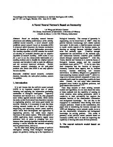
3. Materials and Method In this study, a recognition structure named DBLSTM-WS was used in the classification of ECG signals. In this recognition structure, a new input layer with a wavelet basis was designed differently from standard deep learning layers. In this layer, input signals are decomposed into wavelet levels and transferred to other layers as sequences. For the performance evaluation of this system, the ECG data for five different beat types were segmented from the MIT-BIH arrhythmia database, and the training and test datasets were generated. Later, new deep LSTM networks with different layers and architectures were designed for the classification process. The results obtained from these network models were comprehensively evaluated. 3.1 ECG Data The PhysioBank MIT-BIH arrhythmia [56] database, which is frequently used in studies for the detection of arrhythmic heartbeats, has been used. This database contains heartbeat signals that are just over 30 minutes long for individuals of different sexes and ages. There are 48 records in the database. Experts have annotated the beats in the records stored in the database. In this study, five beats types from different records in the MIT-BIH dataset were used: Normal Sinus Rhythm (NSR), Ventricular Premature Contraction (VPC), Paced Beat (PB), Left Bundle Branch Block (LBBB), and Right Bundle Branch Block (RBBB). Segmented signals from these beat types were used for a period that includes 360 samples. In Fig. 4, the waveforms of the beat types used in the study are given. 9

1.5

mV

1

0.5 0

-0.5

-1 0

50

100

150

200

250

300

350

Samples a) Normal sinus rhythm 2

2

1.5

1

1

mV

mV

0

0.5

-1

0

-2

-3

-0.5 0

50

100

150

200

250

300

-1

350

Samples b) Paced rhythm

0

50

100

150

200

250

300

350

250

300

350

Samples c) VPC rhythm 1

1.5 1

0

mV

mV

0.5

-1

0 -2

-0.5 -1

0

50

100

150

200

250

300

350

Samples d) LBBB rhythm

-3 0

50

100

150

200

Samples e) RBBB rhythm

Figure 4. Waveforms of the beat types used in the study. The beat samples were drawn for a period that includes 360 samples.

3.2 Wavelet Sequences Wavelet transform is a method that is often used to derive meaningful and correct features in the analysis of non-stationary time-series data. This transform method allows a time-scaled decomposition of a signal [57]. The widely used discrete version for WT is called a discrete wavelet transform (DWT). DWT is an approach that reduces the cost of continuous wavelet computation and derives the coefficients by passing the signal through serial digital filters [58]. This decomposition method is also known as multi-resolution analysis. These filter banks consist of high-pass (HP) and low-pass (LP) filters, as shown in Equations (6) and (7).

H



 S[k ] [2n  k ]

L

(6)

h

k  

 S[k ] [2n  k ]

k 

(7)

g

where S is input signal, H and L are the outputs of filters, and

 h and

 g are low-pass and

high-pass filters, respectively. The HP filter outputs include the input signal's detail coefficient (D), and the low-pass filter outputs contain approximate (A) coefficients. The signals passing

10

through the filters are down-sampled by 2 to increase the frequency resolution. In Fig. 5, these decomposition processes are presented level by level.

Main singal

Decomposition Level1

Decomposition Level2 A2 Low-pass

Decomposition Level3 Low-pass

2

High-pass

2

A3

2

A1 Low-pass

2 High-pass

S High-pass

2

2

CD3

CD2

CD1

Figure 5. Discrete wavelet transform multiresolution analysis level by level.

The S input signal is first passed through both the HP and the LP filters to obtain the detail and approximate coefficients at the first level. The obtained approximate coefficient is again filtered to obtain the components of the second level. This process is repeated until a specified level has been reached. Thus, features that contain important information about the input signal are obtained. The detail coefficients represent the frequency-dependent detailed properties of the signal. These filters are connected with a cascade structure to decompose the input signal at different levels. The resolution level in the multi-resolution process depends on the size of the input signal. For example, an input signal with 2n values can be decomposed into n levels. Decomposition can be repeated using appropriate approximations so that the lower resolution components of the signal are obtained. 3.3 Proposed DLSTM Networks In this study, several deep LSTM network models were designed to classify ECG signals. The first of these network models has only unidirectional LSTM types and is briefly called DULSTM. The second model contains two bidirectional LSTM and is briefly called DBLSTM. In addition to these network layers, a new input layer called wavelet sequences (WS) was designed. DULSTM-WS and DBLSTM-WS are the versions of these models that contain WS layers. Fig. 6 shows the block structures that belong to these deep LSTM networks.

11

WS Layer

WS Layer

LSTM

x2

xn

LSTM

LSTM

x1 BLSTM (64)

ULSTM (64)

x1

Level (1-4)

Segmented ECG Signal

Level (1-4)

Segmented ECG Signal

BLSTM (32)

ULSTM (32)

LSTM

xn

LSTM

LSTM

LSTM

LSTM

LSTM

LSTM

Dropout=0.1

Dropout=0.1

LSTM

x2

LSTM

Flatten()

LSTM

LSTM

LSTM

LSTM

LSTM

LSTM

Dense (128)

Dense (128)

Flatten()

Relu

Relu

Dropout=0.2

Dense (5)

Dense (5)

Dropout=0.2

Softmax

y1 y2 y3 y4

Softmax

y1 y2 y3 y4

y5

y5

Figure 6. DLSTM-WS networks used for classification. a) DULSTM-WS has a WS input layer, two unidirectional LSTM layers, and two dense (fully connected) layers. b) DBLSTM-WS has a WS input layer, two bidirectional LSTM, and two dense (fully connected) layers.

At the top of both network models, a wavelet transform based WS layer was placed. In the WS layer, discrete wavelet transform is applied on the segmented input signals. The decomposition process of this layer is applied at the level indicated by the "Level" parameter. For example, if the Level parameter is 3, 3 levels of DWT are applied on the signal. Later the main signal and the detail coefficients of that signal become output as sequences. The wavelet family is another parameter set which can be selected in the WS layer. In this stage, common wavelet families such as Daubechies, Bior, Symlets can be used. After this layer; ULSTM / BLSTM layers, dropout layer, flatten layer and dense layers are placed respectively.

One of the most important challenges in deep neural networks is overfitting. One of the latest solutions to prevent overfitting has recently been the Dropout [59]. At the dropout layer, during training process units are randomly dropped out at the specified rates. This method significantly reduces the overfitting by preventing the units from being too compliance with each other. For this reason, the dropout was placed in two different layers in the designed networks.

12

Optimization of layer parameters in deep networks is a long and time-consuming process. In this study, different combinations of three parameter arrays were examined and applied on the validation set to achieve the highest stability. These arrays are dense layer unit number layer {64, 128, 256, 512}, ULSTM / BLSTM layer numbers array {16, 32, 64, 128} and dropout parameters array {0.1, 0.2, …, 1}. In the proposed networks, after WS layer, one 64 and 32 dimensional ULSTM/BLSTM layers was followed the input, respectively. Dense layers with 128 and 5 units, respectively, were used in the final network layers. In addition, a dropout of 0.1 at the second layer outputs of the networks and 0.2 at the last layer inputs was provided to avoid an overfitting problem. In these networks, each LSTM layers (BLSTM and ULSTM) return the hidden state output for each input time step. Therefore, a flatten layer was placed between LSTMs and dense layers.

Non-linear activation functions are other important components of neural networks which provide important advantages in solving complex problems. Two commonly used activation functions for deep learning are ReLU and softmax. The activation functions of dense layers were selected as ReLU and softmax, respectively. The softmax activation function that can be expressed in Equation (8) used in the last layer provided output values between zero and one.

 ( z) j 

e

zj

 n1 e zn N

for j  1,..., N .

(8)

With these output values, the class that the arrhythmia belongs to is determined. In Table 1, detailed information is provided for each layer of the proposed network models. The model inputs are segmented arrhythmic heartbeat signals. Model outputs are the arrhythmic signals of the five different classes listed above. Table 1. Detailed information for each layer of the proposed network models.

Layers

Layer Names

Layer 1

WS Layer

Main Parameters of Layers 4 Level

Layer 2

ULSTM/BLSTM

64 Unit

Returned_sequences=True, dropout=0.1.

Layer 3

ULSTM/BLSTM

32 Unit

Returned_sequences=True, dropout=0.1.

Layer 4

Flatten

-

-

Layer 5

Dense

128 Unit

Activation=ReLU

Layer 6

Dropout

-

Rate=0.2

Layer 7

Dense

5 Unit

Activation=SoftMax 13

Other Parameters Family: Daubechies (dB6)

4. Experimental Results For the experimental studies, 360 sampled ECG signals segmented for five different arrhythmic heartbeat types were used. This data was selected from the MIT-BIH arrhythmia database. This dataset has a total 7376 original ECG signals without noise removed including 2190 NSR, 510 VPC, 1450 Paced, 1870 LBBB and 1356 RBBB. The distributions of data numbers used in the training, validation and test phases according to classes are given in Table 2. The experimental data were divided as 60% in the training phase, 20% in the validation phase and the remaining 20% in the test phase. The validation dataset was used to tune the parameters and determine the optimal unit numbers of the designed models. During the performance evaluation of the trained model, the test data, which were not used before, were used. Data for testing, validation and training could be used at different ratios, but we preferred this ratio in terms of reducing the complexity of the experimental results. Various parameter settings for the LSTM models designed for classification operation during the experiment were as follows. Batch size was determined as 128, the optimizer selected was the Adam optimizer, and loss function was selected as the categorical cross-entropy. Each experimental result was obtained during 50 epochs to ensure consistent comparisons. Experimental studies were performed on a computer with a 3.40 GHz Intel Xenon E3 1240 v3 processor. Table 2. Number of training and testing ECG samples used in the experimental studies.

Classification Dataset Class

Beat Types

C1 C2 C3 C4 C5

NSR VPC PB LBBB RBBB Total Data

Number of Training Data (60%) 1314 306 870 1122 813 4425

Number of Validation Data (20%) 438 102 290 374 271 1475

Number of Testing Data (20%) 438 102 290 374 272 1476

Total 2190 510 1450 1870 1356 7376

4.1 Experiments on the Standard DLSTMs

In the experimental study, results were first obtained on non-WS layer versions of the network models. The datasets are provided as input for both models as one feature only to ensure they do not contain any additional sequences. Thus, the input data has a sequence size of 4425 × 360 for the training stage. Similarly, the data evaluated in the testing phase has a size of 1475 × 360. 14

Graphs of performance achieved by DULSTM and DBLSTM models on this dataset are given in Fig. 7. 100 90

Accuracy Rate (%)

80 70

60 50

DBLSTM-Train DBLSTM-Val

40

DULSTM-Train DULSTM-Val

30

20 5

10

15

20

25

30

35

40

45

50

Epochs

Figure 7. The recognition performances of standard DULSTM and DBLSTM networks are on singlefeature ECG signals without any additional features. These networks do not have a WS layer.

As can be seen from the graph, DBLSTM network performance is higher than the DULSTM network in terms of both training and validation. On the other hand, the training phase of both networks has not been fully successful. The training performance of the DULSTM network was observed at a maximum of 90.54%, and the validation performance was observed at a maximum of 94.85%. The training performance of the DBLSTM network was 98.92%, and the validation performance was observed at a maximum of 96.81%. When the performance of these networks was evaluated in terms of time cost, the average duration of each epoch of the DBLSTM network lasted 121 seconds, while the value for the DULSTM network was 45 seconds. The confusion matrices for the test data of these models are presented in Table 3 for a more detailed evaluation of the classification performances at the end of the 50th epoch of both networks. Table 3. Confusion matrices of the DULSTM and DBLSTM networks on single-feature ECG signals after the 50th epoch training time.

Class

DULSTM Network C1 C2 C3 C4

C5

Class

DBLSTM Network C1 C2 C3 C4

C5

C1

239

0

0

2

197

C1

244

0

0

0

194

C2

2

74

0

14

12

C2

1

87

0

12

2

C3

0

0

289

1

0

C3

0

0

289

1

0

C4

1

0

0

205

168

C4

5

1

0

282

86

C5

0

0

0

0

272

C5

0

0

0

0

272

Total success rate = 73.10%

Total success rate = 79.53% 15

The performance rates achieved on the ECG test samples of both designed networks were low. Although the recognition rate obtained for the DBLSTM network was higher than for the DULSTM, it is not sufficient for good recognition. These results show that the DBLSTM network is more advantageous for these datasets than the DULSTM network. Both networks have difficulty in identifying the NSR beat type (class-C1), VPC (class-C2) and LBBB (classC4) signals. However, for the PB and RBBB heartbeat type (class- C3 and C5), both networks provided good recognition.

The output of the dense layer with 128 units of network were used to gather information about the characteristics of the features, which was learned from the input signals by the DBLSTM network. The signals from each heartbeat class were applied to the fully-trained network model to obtain 128 features of these signals. Correlation analysis was performed to show the relations of the learned features according to the classes. In Table 4, the results obtained by the correlation analysis were presented. Table 4. Correlation table of learned features at the 5th layer output of the DBLSTM network according to classes.

Heartbeat Types NSR (C1)

NSR (C1) 1

VPC (C2) 0.6753

PB (C3) 0.2921

LBBB (C4) 0.8433

RBBB (C5) 0.7406

VPC (C2) PB (C3)

0.6753 0.2921

1 0.4247

0.4247 1

0.7990 0.4076

0.5059 -0.0035

LBBB (C4) RBBB (C5)

0.8433 0.7406

0.7990 0.5059

0.4076 -0.0035

1 0.6706

0.6706 1

As it can be seen in Table 4, correlation values are consistent with the confusion matrix given in Table 3. The classes with the highest correlation are between C1-C4 (R = 0.8433), C2-C4 (R = 0.7990) and C1-C5 (R = 0.7406). For this reason, the classifier network has difficulty in distinguishing the data of these classes. In order to visualize the features obtained in the dense layer of 128 units of network, the radar plot drawings in Fig. 8 were built using only the values of active neurons in this layer.

16

C2 (VPC)

C1 (NSR)

C3 (PB)

C5 (RBBB)

C4 (LBBB)

Figure 8. Radar plot drawings of active neurons on the 5th layer for each class of the trained DBLSTM network.

In the radar plots, there are overlapping regions among the learned features of the classes in accordance with the correlations. The number of active neurons at the output of this layer is about 45 for each class. Based on these active neurons, the softmax classifier provides an estimate of the class to which the data belong.

4.2 Experiments on DLSTM Networks with a WS Layer

One of the most important components of classifier performance is the characteristics of the input data. Often, these processes are called the feature extraction stage and are hand-crafted. One of the advantages of deep learning architects is that they can operate directly on the data without the need for hand-crafted features. Feature extraction steps using feature extractors can be quite complex. For this reason, in this study, a new layer named the WS layer was designed differently than the feature extraction. This layer is intended to improve the classification performance of DLSTMs. In the WS layer, frequency sub-bands belonging to the signals were obtained for use in the ECG signals classification phase. These sub-bands are presented in sequence to other layers without any additional calculation. The WS layer takes the level information so the signals can be decomposed as parameters. According to this level parameter, sequences are generated in different sub frequency bands belonging to the signals. Fig. 9 shows the waveforms of the sequences generated by the WS layer of the PB class signal for four levels.

17

1

Sequence 1

0.5

mV

0 -0.5 -1 -1.5 -2

0

50

100

150 200 Samples

250

300

350

(a) Main signal 0.03

0.2

Sequence 2

0.02

0.1

mV

mV

0.01

Sequence 3

0

0 -0.1

-0.01

-0.02

0

20

40

60

80 100 Samples

120

140

160

-0.2 0

180

10

20

50 60 Samples

70

80

90

2

Sequence 4

1

mV

0.5

mV

40

(c) 2nd detail band

(b) 1st detail band 1.5 1

30

Sequence 5

0

0 -1

-0.5 -1 0

5

10

15

20

25 30 Samples

35

40

-2 0

45

5

10

15

20

25

Samples

(e) 4th detail band

(d) 3rd detail band

Figure 9. Sequence waveforms produced by the WS layer for 4 levels for an ECG signal of class PB. a) Main input signal b) 1st level detail band output. c) 2nd level detail band waveform. d) 3rd level detail band. e) 4th level detail band.

In this paper, the Daubechies dB6 wavelet member of the wavelet family is used in the WS layer. This wavelet family for ECG signals was chosen because it was indicated in studies in the literature that produced more favorable results [60]. Only the detail coefficients of the main signal were used in the WS layer. Signals decomposed into sub-bands by wavelet transform were transformed into an appropriate form in this layer for the LSTM inputs. As mentioned in previous chapters, wavelet transform performs a down sample using two operations at every level. For this reason, sequences are generated with padding by zero for LSTM inputs in the WS layer. Fig. 10 shows a graphical representation of how a four-sample sequence from a signal were arranged for the LSTM input at the WS layer.

18

CD3 CD4

4th Level Detail Band

3rd Level Detail Band

CD2

WS4

CD1

1st Level Detail Band WS3 WS1 Non-WS Layer

Main Sigal (S)

WS2

Dimensions

2nd Level Detail Band

50

0

100

150

250

200

300

350

Time steps Figure 10. WS layer outputs for LSTM inputs. First dimension includes main signals that has 360 samples. Other dimensions are decompositions of the main signals level by level.

In order to evaluate the effect of the WS layer on classification process, this layer parameter was used by changing from the first level (WS1) to the fourth level (WS4). In terms of understandable experimental results, the number of levels used is shown at the end of the WS layer. For example, in the notation called WS1, the layer parameter is one. This layer outputs the main signal and the 1st level wavelet detail band (WS1 output = [S, CD1]). As the number of levels increases, the number of features of the input signal increases. WS1 provides a twodimensional feature input while WS4 contains five-dimensional (WS4 output = [S, CD1, CD2, CD3, CD4]) feature signals. For each LSTM network designed in this part of the experimental study, the results were evaluated separately. For the DULSTM-WS network, the WS layer parameters were changed from 1 to 4. Both the training and validation results are given in Fig. 11. 100

100

98

98

96

Accuracy Rate(%)

Accuracy Rate(%)

96 94 Train-WS1 Train-WS2 Train-WS3 Train-WS4

92 90 88

Val-WS1 Val-WS2 Val-WS3 Val-WS4

94 92 90

86 88 84

86

82 80 5

10

15

20

25

30

35

40

45

50

Epochs

84 5

10

15

20

25

30

35

40

45

50

Epochs

Figure 11. DULSTM-WS network performances on ECG signals. a) Training accuracy for the WS layer parameters from 1 to 4. b) Validation accuracy for the WS layer parameters from 1 to 4.

19

The DULSTM-WS network provides high performance on ECG signals. The training phase of this network has been successfully completed. In the validation stage, the recognition performance was over 98% for all WS levels. The DULSTM-WS network also provides the best performance in WS3 both the validation and testing stage for ECG signals. The WS3 layer outputs consist of S, CD1, CD2, CD3, and CD4 sequences. The training performance for these layer parameters was 99.61% in the 50th epoch. When examining the test results, it was seen that the DULSTM-WS network generally succeeded to recognize the test data. Similarly, the best performance in the test phase was achieved with the WS3 layer. At the end of the 50th epoch, test data were correctly classified at 99.25%. These results appear to be much better than the standard DULSTM network without the WS layer. WS layer improved DULSTM network performance drastically (+26.15%).

Another experimental study was performed for the

DBLSTM-WS network. Similarly, the WS layer parameters were increased from 1 to 4 for this network and results were obtained. Fig. 12 presents the performance graphs for the training and validation stages when the ECG signals were used as the input for the DBLSTM-WS network. 100

100

98

95

96

Acurracy Rate (%)

Accuracy Rate (%)

90 Train-WS1 Train-WS2 Train-WS3 Train-WS4

85 80 75

94

Val-WS1 Val-WS2 Val-WS3 Val-WS4

92 90

88 86

70 84 65

82

60 5

10

15

20

25

30

35

40

45

50

Epochs

80 5

10

15

20

25

30

35

40

45

50

Epochs

Figure 12. DBLSTM-WS network performances on ECG wavelet sequences. a) Training accuracy for the WS layer parameters from 1 to 4. b) Validation accuracy for the WS layer parameters from 1 to 4.

As can be seen from the performance graphs, the DBLSTM-WS network showed remarkable success on ECG samples containing WS both in the training phase and the validation phase. The training phase for all WS layer levels was successfully completed at the end of the 50th epoch. When examining the performance of the testing data, it was observed that the best recognition performance was achieved with DBLSTM-WS2 at the highest 99.50% and at the end of the 50th epoch with 99.39% accuracy. In addition, the classification performance improved significantly (+19.86%) compared to the standard DBLSTM network without the WS layer. In Table 5, the classification performance on ECG signals with wavelet-based features at

20

the end of 50th epoch of the DULSTM-WS3 and DBLSTM-WS2 networks is given with a confusion matrix.

Table 5. DLSTM-WS networks performance on ECG signals with wavelet based sequences at the end of the 50th epoch.

DULSTM-WS Network (DULSTM-WS3) Class

C1

C2

C3

C4

C5

Precision

Recall

F1-Score

Support

C1

434

1

0

3

0

C1

1.00

0.99

0.99

438

C2

0

100

0

2

0

C2

0.99

0.98

0.99

102

C3

0

0

288

2

0

C3

1.00

0.99

1.00

290

C4

1

0

0

373

0

C4

0.98

1.00

0.99

374

C5

0

0

0

2

270

C5

1.00

0.99

1.00

272

Classification Accuracy Rate (50th epoch) = 99.25%

DBLSTM-WS Network (DBLSTM-WS2) Class

C1

C2

C3

C4

C5

Precision

Recall

F1-Score

Support

C1

436

0

0

2

0

C1

0.99

1.00

0.99

438

C2

0

100

0

2

0

C2

1.00

0.98

0.99

102

C3

0

0

289

1

0

C3

1.00

1.00

1.00

290

C4

4

0

0

370

0

C4

0.99

0.99

0.99

374

C5

0

0

0

0

272

C5

1.00

1.00

1.00

272

Classification Accuracy Rate ( 50th epoch) = 99.39%

As shown in Table 5, the recognition performance of the DULSTM-WS3 network was 99.25% at the end of the 50th epoch. With this network, 4 of the 434 NSR (C1) data and only two of the other classes were misclassified. The signals of heartbeat types were correctly classified at a considerable level with this network. When the DBLSTM-WS3 network was examined, it appeared that this network provided a better recognition performance of 99.39% over all classes. The DBLSTM-WS3 network achieved the lowest recognition performance with NSR (C1) and VPC (C2) classes from the heart rate types. Two samples were wrongly classified for these beat types. Dense layer outputs on the 5th layer of the network are used to examine the characteristics of the learned DBLSTM-WS2 network features. 128 features were obtained for each class in the dense layer output. The correlation values among classes of these features were given in Table 6.

21

Table 6. Correlation values among classes of features learned by the DBLSTM-WS2 network.

Heartbeat Types NSR (C1)

NSR (C1) 1

VPC (C2) 0.2560

PB (C3) 0.0263

LBBB (C4) 0.5746

RBBB (C5) 0.2404

VPC (C2) PB (C3)

0.2560 0.0263

1 0.2401

0.2401 1

0.6537 0.2382

0.3755 -0.0286

LBBB (C4) RBBB (C5)

0.5746 0.2404

0.6537 0.3755

0.2382 -0.0286

1 0.4638

0.4638 1

When the correlation values are examined, it is seen that these values are consistent with the confusion matrix obtained for the test data. Furthermore, DBLSTM-WS2 has lower correlations with the classes than the features learned in the non-WS DULSTM network given in Table 4. The highest correlation values were acquired between the classes C2-C4 (R=0.6537), C1-C4 (R=0.5746) and C4-C5 (R=0.4638). In order to visualize the features learned by this network, outputs belonging to active neurons were used for each class at a dense layer output of 128 units. In Fig. 13, radar plot drawings of active neurons were given for each class.

C2 (VPC)

C1 (NSR)

C3 (PB)

C5 (RBBB)

C4 (LBBB)

Figure 13. Radar plot drawings of active neurons on the 5th layer for each class of the trained DBLSTM-WS2 network.

As it can be seen from these radar plots, class regions are more discrete. Moreover, when compared with the plots given in Fig. 8 for the non-WS layer DBLSMT network, it is seen that the feature size is decreased and the regions are better separated. This result implies that the WS layer reduces the size of the features learned by the deep LSTM networks and it provides 22

more distinguishing features. In addition, the WS layer has performed an augmentation process for inputs so that more effective features can be learned.

To better understand the effectiveness of the proposed DBLSTM-WS classification approach, the best results of the models were compared in the study. These network models are of the form DULSTM, DBLSTM, DULSTM-WS3, and DBLSTM-WS2, respectively. The performance ratios achieved for each network model over the validation data during the 50th epoch are shown in Fig. 14.

100 90

Accuracy Rate (%)

80 70 60 50 DBLSTM (non-WS) DBLSTM-WS2 DULSTM (non-WS) DULSTM-WS3

40 30 20

10 0 5

10

15

20

25

30

35

40

45

50

Epochs Figure 14. Performance comparisons both standard DLSTM and DLSTM-WS networks on the test data. DULSTM and DBLSTM are represented only single-featured ECG signals. DULSTM-WS3 is the DULSTM model with a WS3 layer. DBLSTM-WS3 is the DULSTM model with a WS3 layer.

When the results were examined, it was seen that bidirectional LSTM models are more successful for ECG signals. In addition, network models with the WS layer appear to outperform significantly when compared to standard models. Table 7 presents comprehensive comparisons of significant results from experimental studies. From Table 7 it is seen that the performance of non-WS DLSTM networks was poor on test data. The DULSTM model showed a 73.10% success rate on the ECG data, and the DBLSTM model provided a much better performance with a 79.53% success rate. Although the DBLSTM model is better than the DULSTM model, the model is still not sufficient to recognize the ECG signals. The performance of DLSTM networks with the WS layer has improved significantly, and the performance of the DULSTM-WS2 model with the WS layer reaches to 99.25%. Similarly, the 23

performance on the test data of the non-WS layer DBLSTM network increased from 79.53% to 99.39% with the WS layer (DBLSTM-WS2). Based on these results, the DBLSTM-WS3 network showed the best accuracy performance on the ECG data when the WS layer parameter is 3. In terms of time efficiency, DBLSTM networks require more time than ULSTM networks in the learning process. Table 7. Comprehensive performance comparisons between DLSTM network models. Sequences Size Average Accuracy Rate Deep LSTM Models (samples, times, features) Time (sec) on Test Data Training Testing Per Epoch

DULSTM DULSTM-WS1 DULSTM-WS2 DULSTM-WS3 DULSTM-WS4 DBLSTM DBLSTM-WS1 DBLSTM-WS2 DBLSTM-WS3 DBLSTM-WS4

4425×360×1 4425×360×2 4425×360×3 4425×360×4 4425×360×5 4425×360×1 4425×360×2 4425×360×3 4425×360×4 4425×360×5

1476×360×1 1476×360×2 1476×360×3 1476×360×4 1476×360×5 1476×360×1 1476×360×2 1476×360×3 1476×360×4 1476×360×5

45 46 49 51 50 121 130 132 134 140

73.10 % 98.64% 98.37% 99.25 % 98.30% 79.53 % 98.01 % 99.39 % 98.85 % 98.51 %

5. Discussions There are many studies in the literature on ECG data obtained from the MIT-BIH database. Although the datasets used in these studies are not exactly the same, they are useful for comparison because they are generally classified on ECG signals. In this respect, Table 8 shows a comparison of the proposed methods with other state-of-the-art methods. Yu and Chou [11] performed a classification study using a total of 9800 segmented ECG signals of eight heartbeat types from the MIT-BIH arrhythmia database. They obtained a 98.71% performance by using independent component analysis (ICA) for feature extraction and NN as the classifier. Sahoo et al. [13] have correctly identified 98.39% using DWT and SVM on data from four different beat types obtained from the MIT-BIH database. Martis et al. [31] obtained a 94.52% recognition performance with the Culmant and principal component analyzer (PCA) feature extraction method and NN classifier on five different ECG types in their study. Ubeyli [32], used Lyapunov exponents features and RNN for classification four types of ECG beats obtained from the PhysioBank. Ubeyli achived a 94.72% recognition performance on these beat types. Acharya et al. [34] proposed a CNN model for the automated detection of a normal and MI ECG beats both with noise and without noise. They observed a 95.22% classification 24

performance on ECG beats without noise. Kiranyaz et al. [35] proposed a patient-specific ECG heartbeat classifier with an adaptive implementation of 1D-CNN. In their study, ventricular ectopic beats (VEB) detection accuracy of the proposed system for all training and testing records is found as 99.00%. Zubair et al. [37] obtained 92.70% classification performance for five beats using a CNN-based method for the classification of ECG data obtained from the MITBIH database.

Table 8. Performance comparison of the proposed DBLSTM models with other state-of-the-art studies.

Yu and Chou [11] Sahoo et al. [13] Martis et al. [31]

Number of Beat Types 8 4 5

Ubeyli [32]

4

Acharya et al. [34]

2 5 5 5 5

Study

Kiranyaz et al. [35] Zubair et al. [37] The Proposed Method

Features

Classifier

ICA DWT Cumulant+PCA Lyapunov exponents End-to-end End-to-end End-to-end End-to-end End-to-end

NN SVM NN

Accuracy Rates 98.71 % 98.39% 94.52%

RNN

94.72%

CNN 1D-CNN CNN DULSTM-WS2 DBLSTM-WS3

95.22% 99.00% 92.70% 99.25% 99.39%

In this study, an end-to-end learning structure was employed without any hand-crafted feature extraction in the ECG classification. Bidirectional and unidirectional LSTM models were designed from deep LSTM networks to classify five different heartbeat types. A new WS layer has been designed to improve the performance of DLSTM networks. Thanks to the WS layer, the performance of the DBLSTM network has reached a high recognition performance of 99.39%. The most important advantage of this network model over the hand-crafted methods in the literature is that it provides high performance and does not require any feature extraction stage. Another end-to-end structure is the CNN method. LSTM and CNN methods have advantages over different problems. The complexity of CNN structures depends on convolution process, kernel number and cache unfriendly memory access. On the other hand, LSTMs are located in space and time. Thus, the input length does not affect the network storage requirements [61]. This work presents a new approach to improving the performance of LSTM structures for ECG signal recognition. However, the only disadvantage of the network is the time cost of the training phase, which is a common problem of most deep networks. This extra time cost problem in our method is due to the wavelet transform phase in the WS layer, but this layer increases the recognition performance significantly. Time cost problem can be discarded since a fully trained network is used in real applications. 25

6. Conclusions In this article, the classification of ECG signals was provided using deep LSTM networks, which recently have provided a significant achievement in the field of machine learning. Unidirectional and bidirectional models from deep LSTM networks were created to automatically recognize input data. In the study, a new layer named WS with wavelet transformation base was designed. Through this layer, additional sequences of input signals were obtained using wavelet decomposition on the input signals. These sequences were given as inputs to the LSTM networks. Experimental results were obtained for five different types of beats obtained from the MIT-BIH arrhythmia database. Within these experimental works, many performance comparisons of DBLSTM networks and WS layers have been carried out as well.

When the experimental results were evaluated, it was seen that the performance of the proposed DBLSTM-WS model was drastically successful on ECG signals. The most significant output of the study is that the recognition performance of the DBLSTM network was improved considerably with the designed WS layer. Moreover, through end-to-end learning, significant features related to ECG signals were obtained without any expert intervention or without an additional method, and direct classification was achieved. These results show that the WS layerbased DLSTM network models proposed in the study are effective structures that can be used in other signal classification systems. Future works will include studies with noise added data to measure recognition performance under noisy conditions. In addition, LSTM networks will be combined with other deep learning models to examine different ECG data classification models.

7. References [1] S. Min, B. Lee, & S. Yoon, Deep learning in bioinformatics. Briefings in bioinformatics, 18(2017) 851-869. [2] M. R. Arefin, K. Tavakolian, & R. Fazel-Rezai, QRS complex detection in ECG signal for wearable devices. In Engineering in Medicine and Biology Society (EMBC), 37th Annual International Conference of the IEEE, IEEE, 2015, pp. 5940-5943. [3] H. W. Guo, Y. S. Huang, J. C. Chien, & J. S. Shieh, Short-term analysis of heart rate variability for emotion recognition via a wearable ECG device. In Intelligent Informatics and Biomedical Sciences (ICIIBMS), 2015 International Conference on, IEEE, 2015, pp. 262-265. [4] V.S. Chouhan, S.S Mehta, Threshold-based detection of P and T-wave in ECG using new feature signal, International Journal of Computer Science and Network Security, 8 (2008) 144-153. 26

[5] S. Mahmoud, A. Bamakhramah, & S. Al-Tunaiji, Six order cascaded power line notch filter for ECG detection systems with noise shaping, Circuits Syst. Signal Process. J., 1–17 (2014), doi:10.1007/s00034-014-9761-1. [6] E. Pasolli, & F. Melgani, Active learning methods for electrocardiographic signal classification. IEEE Transactions on Information Technology in Biomedicine, 14(2010) 1405-1416. [7] Z. Zidelmal, A. Amirou, M. Adnane, & A. Belouchrani, QRS detection based on wavelet coefficients. Computer methods and programs in biomedicine, 107(2012) 490-496. [8] M. A. Kabir, & C. Shahnaz, Denoising of ECG signals based on noise reduction algorithms in EMD and wavelet domains, Biomedical Signal Processing and Control, 7(2012) 481-489. [9] U. Raghavendra, H. Fujita, A. Gudigar, R. Shetty, K. Nayak, U. Pai, ... & U. R. Acharya, Automated technique for coronary artery disease characterization and classification using DD-DTDWT in ultrasound images, Biomedical Signal Processing and Control, 40(2018) 324-334. [10] S. L. Oh, M. Adam, J.H. Tan, Y. Hagiwara, V.K. Sudarshan, J.E.W. Koh, ... & E.Y. Ng , Automated identification of coronary artery disease from short-term 12 lead electrocardiogram signals by using wavelet packet decomposition and common spatial pattern techniques, Journal of Mechanics in Medicine and Biology, 17(2017) 1740007. [11] S.N. Yu, K.T. Chou, Integration of independent component analysis and neural networks for ECG beat classification, Expert Syst. Appl. 34 (2008) 2841-2846. [12] O.T. Inan, L. Giovangrandi, G.T. Kovacs, Robust neural-network-based classification of premature ventricular contractions using wavelet transform and timing interval features, IEEE Transactions on Biomedical Engineering, 53 (2006) 2507-2515. [13] S. Sahoo, B. Kanungo, S. Behera, S. Sabut, Multiresolution wavelet transform based feature extraction and ECG classification to detect cardiac abnormalities, Measurement, 108 (2017) 55-66. [14] M. Thomas, M.K. Das, S. Ari, Automatic ECG arrhythmia classification using dual tree complex wavelet based features, AEU-International Journal of Electronics and Communications, 69 (2015) 715721. [15] R.J. Martis, U.R. Acharya, L.C. Min, ECG beat classification using PCA, LDA, ICA and discrete wavelet transform, Biomedical Signal Processing and Control, 8 (2013) 437-448. [16] Y. Kutlu, D. Kuntalp, Feature extraction for ECG heartbeats using higher order statistics of WPD coefficients, Comput. Methods Progr. Biomed., 105 (2012) 257–267. [17] P. Raman, S.M. Ghosh, Classification of Heart Diseases based on ECG analysis using FCM and SVM Methods, International Journal of Engineering Science, 6(2016) 6739-6744. [18] A. F. Khalaf, M. I., Owis, & I. A. Yassine, A novel technique for cardiac arrhythmia classification using spectral correlation and support vector machines. Expert Systems with Applications, 42(2015) 8361-8368. [19] P. Melin, J. Amezcua, F. Valdez, & O. Castillo, A new neural network model based on the LVQ algorithm for multi-class classification of arrhythmias. Information sciences, 279(2014) 483-497. [20] M. K. Gautam, & V. K. Giri, An approach of neural network for electrocardiogram classification, APTIKOM Journal on Computer Science and Information Technologies, 1(2016) 115-123. 27

[21] J. Kim, H. Shin, Y. Lee, M. Lee, Algorithm for classifying arrhythmia using Extreme Learning Machine and principal component analysis, Conf. Proc. IEEE Eng. Med. Biol. Soc., 2007, pp. 32573260. [22] Y. Bengio, Learning deep architectures for AI, Foundations and Trends in Machine Learning, 2(2009) 1-127. [23] Y. LeCun, L. Bottou, Y. Bengio, P. Haffner, Gradient-based learning applied to document recognition, Proceedings of the IEEE, 86(1998), 2278-2324. [24] M. Coşkun, A. Uçar, Ö. Yıldırım, & Y. Demir, Face Recognition Based on Convolutional Neural Network, International Conference on Modern Electrical and Energy Systems, 2017. [25] A. Uçar, Y. Demir, & C. Güzeliş, Object recognition and detection with deep learning for autonomous driving applications, SIMULATION, 9 (2017) 759-769. [26] S. Ren, K. He, R. Girshick, X. Zhang, & J. Sun, Object detection networks on convolutional feature maps, IEEE transactions on pattern analysis and machine intelligence, 39(2017) 1476-1481. [27] Ö. Yildirim, A. Uçar, U.B. Baloglu, Recognition of Real-World Texture Images Under Challenging Conditions With Deep Learning, ASYU 2017, 52. [28] A. Krizhevsky, I. Sutskever, & G. E. Hinton, 2012, Imagenet classification with deep convolutional neural networks, In Advances in neural information processing systems, 2012, pp. 1097-1105. [29] P. Rajpurkar, A. Y. Hannun, M. Haghpanahi, C. Bourn, & A. Y. Ng, Cardiologist-level arrhythmia detection with convolutional neural networks. arXiv preprint arXiv:1707.01836, 2017. [30] S.Chauhan, & L. Vig, Anomaly detection in ECG time signals via deep long short-term memory networks, Data Science and Advanced Analytics (DSAA), IEEE International Conference on, IEEE, 2015. [31] M. M. Al Rahhal, Y. Bazi, H. AlHichri, N. Alajlan, F. Melgani, & R. R. Yager, Deep learning approach for active classification of electrocardiogram signals. Information Sciences, 345(2016) 340354. [32] E. D. Übeyli, Recurrent neural networks employing Lyapunov exponents for analysis of ECG signals, Expert Systems with Applications, 37(2010) 1192-1199. [33] R. Salloum, & C. C. J. Kuo, ECG-based biometrics using recurrent neural networks. In Acoustics, Speech and Signal Processing (ICASSP), IEEE International Conference on, IEEE, 2017, pp. 20622066. [34] U. R. Acharya, H. Fujita, S. L.Oh, Y. Hagiwara, J. H. Tan, & M. Adam, Application of deep convolutional neural network for automated detection of myocardial infarction using ECG signals. Information Sciences, 415(2017) 190-198. [35] S. Kiranyaz, T. Ince, & M. Gabbouj, Real-time patient-specific ECG classification by 1-D convolutional neural networks. IEEE Transactions on Biomedical Engineering, 63(2016) 664-675. [36] U. R. Acharya, H. Fujita, O.S. Lih, Y. Hagiwara, J.H. Tan, & M. Adam, Automated detection of arrhythmias using different intervals of tachycardia ECG segments with convolutional neural network, Information sciences, 405(2017), 81-90.

28

[37] M. Zubair, J. Kim, & C. Yoon, An automated ECG beat classification system using convolutional neural networks. IEEE 6th International Conference on IT Convergence and Security (ICITCS), (2016) 1-5. [38] Z. Wu, X. Ding, G. Zhang, X. Xu, X. Wang, Y. Tao, & C. Ju, A novel features learning method for ECG arrhythmias using deep belief networks, IEEE 6th International Conference on Digital Home (ICDH), (2016) 192-196. [39] J. H. Tan, Y. Hagiwara, W. Pang, I. Lim, S.L. Oh, M. Adam, ... & U.R. Acharya, Application of stacked convolutional and long short-term memory network for accurate identification of CAD ECG signals, Computers in Biology and Medicine, (2018). [40] B. Hwang, J. You, T. Vaessen, I. Myin-Germeys, C. Park, & B.T. Zhang, Deep ECGNet: An Optimal Deep Learning Framework for Monitoring Mental Stress Using Ultra Short-Term ECG Signals, Telemedicine and e-Health, (2018). [41] P. Warrick, & M.N. Homsi, Cardiac Arrhythmia Detection from ECG Combining Convolutional and Long Short-Term Memory Networks, (2018), arXiv preprint arXiv:1801.10033. [42] J. Yang, Y. Bai, F. Lin, M. Liu, Z. Hou, & X. Liu, A novel electrocardiogram arrhythmia classification method based on stacked sparse auto-encoders and softmax regression, International Journal of Machine Learning and Cybernetics, (2017) 1-8. [43] T. Mikolov, & G. Zweig, Context dependent recurrent neural network language model, SLT, 12 (2012) 234-239. [44] A. Graves, A. R. Mohamed, & G. Hinton, Speech recognition with deep recurrent neural networks, In Acoustics, Speech and Signal Processing (ICASSP), 2013 IEEE International conference on, IEEE, 2013, pp. 6645-6649. [45] A. Karpathy, & L. Fei-Fei, Deep visual-semantic alignments for generating image descriptions. In Proceedings of the IEEE Conference on Computer Vision and Pattern Recognition, 2015, pp. 31283137. [46] N. Kalchbrenner, & P. Blunsom, Recurrent continuous translation models. In EMNLP, 3(2013), p. 413. [47] J. J. Hopfield, Neural networks and physical systems with emergent collective computational abilities. In Spin Glass Theory and Beyond: An Introduction to the Replica Method and Its Applications, 1987, pp. 411-415. [48] M.I. Jordan, (1986), Serial order: A parallel distributed processing approach (Tech. Rep. No. 8604), San Diego: University of California, Institute for Cognitive Science, 1986. [49] J. L. Elman, Finding structure in time, Cognitive science, 14(1990), 179-211. [50] S. Hochreiter, & J. Schmidhuber, Long short-term memory, Neural computation, 9(1997) 17351780. [51] H. Sak, A. Senior, & F. Beaufays, Long short-term memory recurrent neural network architectures for large scale acoustic modeling, In Fifteenth Annual Conference of the International Speech Communication Association, 2014. 29

[52] C. Olah, Understanding LSTM networks. GITHUB blog, Access on January 2018. [53] S. Yan, Understanding LSTM networks. Online. Accessed on January 2018. [54] M. Schuster, and K. K. Paliwal, Bidirectional recurrent neural networks, IEEE Transactions on Signal Processing, 45(1997) 2673–2681. [55] A. Graves, & J. Schmidhuber, Framewise phoneme classification with bidirectional LSTM and other neural network architectures, Neural Networks, 18(2005), 602-610. [56] R. Mark, G. Moody, http://ecg.mit.edu/dbinfo.html

MIT-BIH

Arrhythmia

Database,

May.1997,

Available

at:

[57] J. S. Murguia, & H. C. Rosu, Discrete wavelet analyses for time series, In Discrete Wavelet Transforms-Theory and Applications. InTech, 2011. [58] S. Mallat, A Wavelet Tour of Signal Processing, Academic Press, 1999. [59] N. Srivastava, G. Hinton, A. Krizhevsky, I. Sutskever, and R. Salakhutdinov, Dropout: A simple way to prevent neural networks from overfitting, Journal of Machine Learning Research, 15(2014) 1929–1958. [60] I. Güler, E.D. Ubeyli, ECG beat classifier designed by combined neural network model, Pattern recognition, 38 (2005) 199-208. [61] E. Tsironi, P. Barros, C. Weber, & S. Wermter, An analysis of convolutional long short-term memory recurrent neural networks for gesture recognition, Neurocomputing, 268 (2017) 76-86.

30