A Numerical Method Based on the Parametric Variational Principle for ...
Recommend Documents
Nov 24, 2010 - FA] 24 Nov 2010. ON EKELAND'S ... nice paper [9], under the assumption that the functional does not increase by polariza- tion, the ... 2010 Mathematics Subject Classification. 35A15 .... Paris Sér. 275 (1972), 1057-1059.
Palatini variation of this Lagrangian yields the geometrical Einstein-Maxwell affine ... Einstein-Maxwell field equations by the identification of the Maxwell field ...
Jan 27, 2013 - Li Yao,1 Yun-Jie Yang,1 and Xing-Wei Zhou1,2. 1 Department of Mathematics, Kunming University, 2 Puxin Road, Kunming, Yunnan 650214, ...
Oct 25, 2015 - 2College of Mechanical and Power Engineering, Chongqing University of Science and Technology, ... machinery, including multicomponent coupling vibration, ...... monitoring of rotating machinery,â Structural Health Monitor-.
Apr 29, 2012 - arXiv:1104.0866v8 [physics.flu-dyn] 29 Apr 2012. 1. A Variational Principle for Dissipative Fluid Dynamics. Hiroki Fukagawaâ) and Youhei ...
Feb 5, 2008 - + div (Ïi ui)=0. (1.2). Here [ t1, t2] is a time interval , D is a domain in the physical space, the potential. W(Ï1 ,Ï2 ,w) is connected with the ...
We first formulate the principle for paraxial waves and then generalize it to
arbitrary ... derive a new variational principle in optics that relates the phase and
the ...
Apr 2, 2013 - London, WC1E 6BT, United Kingdom. E-mail: [email protected]. A recently proposed variational approach for general relativity where, ...
Oct 25, 2004 - [5] Hans Föllmer, On entropy and information gain in random fields, Z. ... [6] Hans-Otto Georgii, Gibbs measures and phase transitions, ...
Jul 7, 2009 - âCardinal Stefan Wyszynski University, ul. Dewajtis 5, Warszawa, Poland and Systems. Research Institute, Polish Academy of Sciences, ul.
age segmentation and non-rigid registration using prior shape and intensity infor- mation is ... gion matching and segmentation with free boundary conditions in [23], but the model .... is used as an initial contour and the domain is taken as.
Feb 7, 2008 - gravitating spherical shell of mass m can be introduced with the ... If there is an exterior gravitational field then the kinetic and potential energy ...
(p)=(x(p),y(p))(p â [0, 1]) be a differentiable parameterized curve, called ..... Meyer, C., Boes, J., Kim, B., and Bland, P. : Probabilistic Brain Atlas Construction: Thin- ... Richard, F. and Cohen, L. : A New Image Registraton Technique with Fre
numeric methods. In this paper, a new method, which is generalized from finite difference method, has been provided to solve the delay differential equations.
Aug 20, 2007 - Simon Anders 1, Hans J. Briegel 1,2, Wolfgang Dür 1,2. 1 Institut für ...... This part was bound to the main Python code using SWIG [B+]. For the ...
decomposition (VMD) method is introduced into the bolt detection signal ... such as the Short-time Fourier transform, Gabor transform, Wigner-Ville ..... [7] Griffin D, Lim J S. Signal estimation from modified short-time Fourier transform[J].
The Eulerian variational principle in a rotating coordinate system is briejly reviewed. ... So far the application of Hamilton's principle in hydrodynamics has not been used ... The present author also considers that previous derivations are all.
May 20, 2013 - [14] M. A. Khan, Siraj-ul-Islam, I.A. Tirmizi, E.H. Twizell, S. Ashraf, A class of methods based on non-polynomial sextic spline functions for the ...
Feb 2, 1999 - entirely freeâ and formulated the virtual work by summing up the contributions .... Subdomain linking is done through the displacement ubi of the.
Jul 31, 2011 - Method of Fundamental Solutions for the Analysis of Sound Scattering ... CICC, Department of Civil Engineering, University of Coimbra, Pinhal de Marrocos, ... Here, a hybrid numerical-analytical model is proposed to address.
solve the EulerâLagrange equation obtained, and the optimal control law is easily ... For analytical methods, dynamic programming (DP) is a method in very ...
Oct 31, 2016 - 2 and Anthony Nouy3. 1 Departamento de Ciencias Fısicas, Matemáticas y de la Computación. Universidad CEU Cardenal Herrera.
Mar 30, 2004 - School of Mechanical Engineering ... boundaries between the regions of distinct material classes are embedded in their ..... ase, the vector.
A Numerical Method Based on the Parametric Variational Principle for ...
Dec 12, 2017 - Faculty of Vehicle Engineering and Mechanics, Dalian University of Technology, Dalian 116023, China ... it is becoming an increasingly popular method of travel. With the rapid development of ... Volume 2018, Article ID 7208045, 21 pages ...... 121. 116.99. 9.62. Elastic modulus (MPa). 1.2 × 10⁵. 1.2 × 10⁵.
Hindawi Shock and Vibration Volume 2018, Article ID 7208045, 21 pages https://doi.org/10.1155/2018/7208045
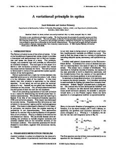
1. Introduction High-speed railway is an inexpensive, secure, comfortable, and efficient mode of transportation, even more time-saving and cheaper than airlines for relatively short journeys. Thus, it is becoming an increasingly popular method of travel. With the rapid development of high-speed railway technology, train speeds are becoming increasingly high. To guarantee that trains run safely and stably after speed-up, the current collection performance directly influenced by the dynamic performance of the pantograph-catenary system must be improved. The catenary consists of a messenger wire, a contact wire, periodically placed droppers, supporting brackets, and registration arms, as shown in Figure 1. The messenger wire is supported by the supporting brackets, and the registration arms are installed on the contact wire. The messenger wire and the contact wire are connected by the droppers. The pantograph, which consists of a pan-head, an upper frame, and a lower frame acts as a current collector between the catenary and the electric train.
A large number of studies have examined the dynamic behavior of the pantograph-catenary system. An overview of the methods used to describe the dynamic behavior of the pantograph-catenary system was introduced by Poetsch et al. [1]. Wu [2, 3] established a finite element model for determining the initial state of the simple stitched catenary and carried out numerical evaluations of the system’s current collection by using Newmark’s method, developing a model through the finite element method (FEM). Wu and Brennan [4, 5] developed a single-degree-of-freedom (SDOF) model of a combined pantograph-catenary system to study its dynamics behavior and presented an analytical approach to the solution of the system. Based on the penalty method, Collina and Bruni [6] developed a procedure for simulating the contact between the contact wire and the pantograph. Arnold and Simeon [7, 8] established a realistic and detailed pantographcatenary system model and coupled DAEs and PDEs to simulate the interaction of the pantograph and the catenary. A simplified catenary model and linear spring-mass-damper model of the pantograph were used to perform a sensitivity analysis
2
Shock and Vibration
Bracket Messenger wire Registration arm Contact wire
Dropper Pantograph
Figure 1: A simple stitched catenary system.
of the pantograph [9, 10]. Because of the intrinsic nonlinear behavior of the catenary, Lopez-Garcia et al. [11] used the Newton-Raphson method to obtain the initial equilibrium state of the catenary, which is the premise and foundation for simulating the dynamic behavior of the pantograph-catenary system. Lopez-Garcia et al. [12] proposed an improvement of the simplified models by considering the effects of stiffness and contact modeling. Rauter et al. [13] established a mixed model of the pantograph-catenary system by using the FEM and multibody dynamics; they then used a constant-timestep Newmark-type of integration algorithm for dynamic analysis of the catenary model and used a variable order and variable-time-step Gear integration algorithm for dynamic analysis of a multibody pantograph model. Dahlberg [14] provided a closed-form solution for the deflection of a contact wire caused by a moving force. Metrikine and Bosch [15] proposed an analytical method for calculating the steadystate response of a two-level catenary to a uniformly moving pantograph based on the Fourier transformation. Zhou and Zhang [16] established a pantograph-catenary model including a support wire, an assistant wire, a contact wire, droppers, and a spring-stiffness-mass pantograph; they then studied the dynamic behavior of the system based on a direct integration method involving the contact element. Cho [17] proposed a formulation for a nonlinear dropper and the proper implementation of a time-integration method for the FEM of the pantograph-catenary system and validated the formulation experimentally. Lopez-Garcia et al. [18] compared the cable slackening model and cable-only taut model and demonstrated the importance of cable slackening in stiffness computation. Commercial software was used to establish the finite element model of the pantograph-catenary system and to simulate its dynamic behavior [19, 20]. Cho et al. [21] presented a modified SDOF dynamic system with a time-varying stiffness to include the pre-sag’s effect on the dynamic interaction of the pantograph-catenary. To obtain more realistic simulation results, an advanced 3D model for studying and simulating the pantograph-catenary system was established by Benet et al. [22]. Van et al. [23] introduced catenary geometry irregularity, catenary wear, and transient aerodynamic forces into pantograph-catenary dynamic simulations. A moving mesh method was presented by JimenezOctavio et al. [24] to analyze the dynamic interaction of the
pantograph-catenary system. Gregori et al. [25] presented a highly computational-cost-saving approach (Offline/Online approach) to simulate the pantograph-catenary dynamic interaction. Bruni et al. [26] described the results of a voluntary benchmark initiative concerning the simulation of pantograph-catenary interaction, which can be used to demonstrate the accuracy of numerical methodologies and simulation models. These studies suggest that wave reflection and the variation of the stiffness are the main causes of contact force variation when a pantograph moves at a constant speed. Both the variation of the stiffness and wave reflection are directly affected by droppers. To simulate the dynamic behavior of the pantograph-catenary system accurately, the nonlinear dropper must be considered. The dynamic behavior of the pantograph-catenary system consists of two main parts, the vibration of the pantograph and the vibration of the catenary caused by the moving pantograph. First, the pantograph and the contact wire will be in one of two states: contact or separation. The contact state and the value of the contact force directly affect the dynamic behavior of the pantograph-catenary system. Therefore, determining the contact state between the pantograph and the contact wire is one of the key problems that must be addressed in simulating the dynamic behavior of the pantograph-catenary system. Second, the dropper may be slack during the passage of the pantograph and then return to the tension state after the pantograph passes. The dropper will experience no force when it is slack, whereas when it is under tension, the force will be positive. The slackening of a dropper reflects a strong nonlinear characteristic. Thus, another important problem associated with the dynamic simulation of the pantograph-catenary system is determining the tension state or compression state of every dropper at every time step. Finally, the significant wave effect of the contact wire subjected to a moving pantograph at high speed makes precise simulation more difficult, particularly when contact problems and nonlinear droppers are involved. The FEM is typically combined with a time-integration method to analyze the response of the catenary to a moving pantograph. In the case of high velocity, both the discrete elements and the time step for integration must be small, which leads to enormous computational requirements and poor efficiency. Thus, an efficient time-integration method for computing the response of the catenary subjected to a moving pantograph must be developed. Determining the contact state between the pantograph and the contact wire and the tension or compression state of a nonlinear dropper are both essentially contact problems. Both the formulations of nonlinear droppers in the catenary and the contact between the pantograph and the contact wire will be proposed based on the parametric variational principle (PVP) [27], which provides a distinct advantage in achieving good convergence for certain strongly nonlinear numerical analyses. By using the proposed method, the contact force can be accurately computed, and the tension or compression state of nonlinear droppers can be accurately determined. Based on the periodicity of the catenary and the precise integration method (PIM) [28], an efficient timeintegration algorithm for computing its responses will thus
Shock and Vibration
3
···
···
···
···
···
(a)
p
L
Bracket
m1
Messenger wire
mbr , kbr
Tm
Tm
k1
m , EIm
m2
Dropper H
···
d , Ed A d
Contact wire
c , EIc Registration arm
k2
L1
mre , kre
p ···
L2 (b)
c2 m3
Tc
Tc
c1
k3 P0
Ld
c3
Roof of train (c)
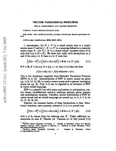
Figure 2: The model of the pantograph-catenary system: (a) the pantograph-catenary system, (b) a unit cell of the catenary, and (c) the pantograph.
be established. In this method, the matrix exponential of only one unit cell of the catenary need be computed, which greatly improves the computational efficiency. This paper is organized as follows. In Section 2, the dynamic model of the pantograph-catenary system is described. Section 3 provides formulations for the nonlinear dropper and the contact between the pantograph and the contact wire. A numerical time-domain integral method for determining the dynamic responses of the pantographcatenary system is developed in Section 4. In Section 5, the nonlinear problems associated with contact and the nonlinear droppers are converted to a standard complementarity problem. Section 6 presents 3 validations. The first is for the contact model between a pantograph and a contact wire, the second is for the nonlinear dropper model, and the last one is for the proposed procedure. The dynamic behaviors of the pantograph-catenary system are then discussed in Section 7, including the variation of the contact forces and the elongation of the nonlinear droppers. Finally, Section 8 presents the main conclusions.
2. The Model of the Pantograph-Catenary System The model of the pantograph-catenary system is shown in Figure 2(a), which consists of a catenary and a pantograph. The catenary consists of a messenger wire, a contact wire,
periodically placed droppers, supporting brackets, and registration arms (see Figure 2(b)). Any part of the catenary that corresponds to the subsection between two successive registration arms can be regarded as a unit cell, as shown in Figure 2(b). The span length and the structure height of the catenary are 𝐿 and 𝐻, respectively. The pretension, linear mass, and flexural rigidity of the messenger wire are 𝑇𝑚 , 𝜌𝑚 , and 𝐸𝐼𝑚 , respectively. The pretension, linear mass, and flexural rigidity of the contact wire are 𝑇𝑐 , 𝜌𝑐 , and 𝐸𝐼𝑐 , respectively. There are 𝑛𝑑 droppers at positions 𝐿 𝑖 (𝑖 = 1, 2, . . . , 𝑛𝑑 ) in a unit cell, and the linear mass, tensile modulus, and sectional area of a dropper are 𝜌𝑑 , 𝐸𝑑 , and 𝐴 𝑑 , respectively. The mass and stiffness of the supporting bracket and the registration arm are 𝑚sb , 𝑘sb , 𝑚ra , and 𝑘ra , respectively. The pantograph can be modeled as a three-level mass-spring-damper system [17], as shown in Figure 2(c). The mass, stiffness, and damping of the pan-head, upper frame, and lower frame are 𝑚1 , 𝑚2 , 𝑚3 , 𝑘1 , 𝑘2 , 𝑘3 , 𝑐1 , 𝑐2 , and 𝑐3 , respectively. The static uplift force is 𝑃0 , and the contact force is denoted by 𝜆 𝑝 . Theoretically, the catenary is infinitely extended. However, the wave in the catenary caused by the contact due to a moving pantograph can be transferred to a finite distance for a period of time. Thus, a catenary including sufficient number of unit cells is used for simulation. Assuming that the catenary includes 𝑁 unit cells, there are 𝑁 × 𝑛𝑑 droppers, 𝑁 + 1 supporting brackets, and 𝑁 + 1 registration arms.
4
Shock and Vibration
Because of negligible displacements in the lateral direction, considering only vertical displacements, a plane model of the pantograph-catenary system can be obtained. The messenger wire can be modeled as an Euler-Bernoulli beam. Assuming that the pretension applied to the messenger wire is constant and the slope of the messenger wire is small, the equilibrium equation of the messenger wire can be derived from the literature [17] as 𝜌𝑚
under tension, the force will be positive. Therefore, the axial stiffness 𝐸𝐴 𝑑,𝑘 will be positive when the dropper is under tension and will be zero when the dropper is slack; that is, 𝐸 𝐴 , 𝑙𝑘 > 𝑙0,𝑘 , 𝐸𝐴 𝑑,𝑘 = { 𝑑 𝑑 0, 𝑙𝑘 ≤ 𝑙0,𝑘 ,
𝑁+1
+ ∑ 𝛿 (𝑥 − (𝑖 − 1) 𝐿) 𝑓sb,𝑖 , 𝑖=1
𝜕𝑦𝑚 𝑦𝑚 (𝑥, 0) = 𝑦𝑚,0 (𝑥) , (𝑥, 0) = 0, 𝜕𝑡 where subscript 𝑚 denotes the messenger wire, 𝑦𝑚 denotes vertical displacement, 𝑔 denotes gravitational acceleration, 𝛿(𝑥) denotes a Dirac delta function, 𝑓𝑚,𝑘 denotes an external force caused by a dropper, 𝑓sb,𝑖 denotes an external force caused by a supporting bracket, and 𝑦𝑚,0 (𝑥) denotes the initial displacement of the messenger. The droppers serve as connectors between the messenger wire and contact wire when they are under tension. The equilibrium equation of the 𝑘th dropper can be described as 𝜌𝑑
where 𝑙0,𝑘 is the original length of the 𝑘th dropper. Eq. (4) indicates that the stiffness is associated with the state of tension or compression of the dropper. To reflect the nonlinear characteristic of the dropper, the tension state or compression state must be determined accurately. The contact wire can be modeled as an Euler-Bernoulli beam. Assuming that the pretension applied to the contact wire is constant and the slope of the contact wire is small, the equilibrium equation of the contact wire can be derived from the literature [17] as 𝜌𝑐
where subscript 𝑑 denotes the dropper, 𝑦𝑑,𝑘 denotes vertical displacement of the 𝑘th dropper from the equilibrium profile, 𝐸𝐴 𝑑,𝑘 denotes the axial stiffness of the 𝑘th dropper, 𝑙𝑘 denotes the length of the 𝑘th dropper, 𝑓𝑚,𝑘 denotes an external force caused by the messenger wire, 𝑓𝑐,𝑘 denotes an external force caused by the contact wire, and 𝑦𝑑,𝑘,0 (𝑦) denotes the initial displacement of the 𝑘th dropper. If a dropper is regarded as a bar with the same tensile and compressive modulus, the axial stiffness 𝐸𝐴 𝑑,𝑘 will be a positive constant regardless of whether the dropper is under tension or compression. However, the dropper cannot operate under compression in engineering practice. During the passage of a pantograph, the dropper may slacken (see Figure 3) and then return to tension. The slackening of the dropper reflects a strong nonlinear characteristic. There will be no force on the dropper when it is slack, while when it is
𝑦𝑐 (𝑥, 0) = 𝑦𝑐,0 (𝑥) ,
𝜕𝑦𝑐 (𝑥, 0) = 0, 𝜕𝑡
(6)
where subscript 𝑐 denotes the contact wire, 𝑦𝑐 denotes vertical displacement, 𝑓𝑐,𝑘 denotes an external force caused by a dropper, 𝑓ra,𝑗 denotes an external force caused by a registration arm, 𝜆 𝑝 denotes a contact force caused by a pantograph, 𝑉 denotes the speed of a moving pantograph, and 𝑦𝑐,0 (𝑥) denotes the initial displacement of the contact wire. Modeling the pantograph as a three-level mass-springdamper system (see Figure 2(c)), the equation of motion for the pantograph can be derived from the literature [17] as 0 𝜆𝑝 { { { } { } } } M𝑝 ÿ𝑝 + C𝑝 ẏ𝑝 + K𝑝 y𝑝 = { 0 } + G𝑝 − { 0 } , { } { } {𝑃0 } {0} y𝑝 (0) = y𝑝,0 , ẏ𝑝 (0) = 0,
(7)
Shock and Vibration
5
where 𝑚1
[ M𝑝 = [
] ],
𝑚2
𝑚3 ]
[
𝑘1 −𝑘1 [−𝑘 𝑘 + 𝑘 K𝑝 = [ 1 1 2 [
−𝑘2
𝑐1 −𝑐1 [−𝑐 𝑐 + 𝑐 C𝑝 = [ 1 1 2 [
−𝑐2
−𝑘2 ] ], 𝑘2 + 𝑘3 ] −𝑐2 ] ],
(8)
𝑐2 + 𝑐3 ]
{𝑦𝑝,1 } { } { } y𝑝 = {𝑦𝑝,2 } , { } { } {𝑦𝑝,3 } 𝑚1 𝑔 { } { } G𝑝 = − {𝑚2 𝑔} , { } {𝑚3 𝑔} where subscript 𝑝 denotes the pantograph; 𝑦𝑝,1 , 𝑦𝑝,2 , and 𝑦𝑝,3 denote vertical displacements of the pan-head, upper frame, and lower frame, respectively; and y𝑝,0 denotes the initial displacement of the pantograph. If the pantograph contacts the contact wire, the contact force should be positive; that is, 𝜆 𝑝 > 0; otherwise, 𝜆 𝑝 = 0. Determining the contact state between the pantograph and the contact wire is a key problem in simulating the dynamic behavior of the pantograph-catenary system, which consists in determining whether the pantograph contacts the contact wire and computing the value of the contact force. In addition, to obtain precise simulation results for the catenary with a pantograph moving at high speed, the number of unit cells must be large; therefore, a highly computationally efficient time-domain integration method should be developed for numerical simulation. By analyzing the model of the pantograph-catenary system, simulating its dynamic behavior at high-speed can be summarized as involving the following three key problems: accurately simulating the nonlinear behavior of the droppers; determining the contact state between the pantograph and the contact wire and computing the value of the contact force; and developing an efficient time-integration method for simulating the dynamic behavior of the pantograph-catenary system. In this paper, the formulations for the nonlinear droppers and for the contact between the pantograph and the contact wire will be proposed based on PVP, and a numerical time-integration algorithm for computing the response of the catenary will be developed based on PIM.
3. PVP for the Pantograph-Catenary System 3.1. PVP for the Nonlinear Dropper. The droppers connect the messenger wire and contact wire when they are under
tension. The dropper may be slack when a pantograph passes it and return to tension after the pantograph leaves. The dropper cannot operate if it is slack; that is, if a dropper slackens, it no longer serves as a connector between the messenger wire and the contact wire. Therefore, at every time step, the tension or compression state of every dropper must be determined. PVP proposed by Zhong and Zhang [27] has been proved to be advantageous for convergence for certain strong nonlinear numerical analyses, such as contact and piecewise linear analyses [29–31]. Therefore, in this paper, the nonlinear droppers are described by PVP, which converts the nonlinear problem to a linear complementarity problem. The tension or compression state of the nonlinear dropper can be accurately determined by the proposed method. A dropper is modeled as a bilinear mass-spring-damper with a bilinear stiffness 𝑘𝑑 , a damper 𝑐𝑑 , and two lumped masses attached to the ends to represent the mass summed for half of the dropper 𝑚𝑑 /2 and its clamp 𝑚𝑠 , respectively, as shown in Figure 4(a). The constitutive relation of the bilinear spring (see Figure 4(b)) can be described as 𝑓𝑑 = 𝑘𝑑 Δ𝑢,
(9)
where 𝑓𝑑 is the axial force, Δ𝑢 is the elongation of the dropper, and 𝑘𝑑 is the stiffness determined by the signs of Δ𝑢; that is, (+) {𝑘𝑑 , Δ𝑢 ≥ 0, 𝑘𝑑 = { (−) 𝑘 , Δ𝑢 < 0. { 𝑑
(10)
If 𝑘𝑑(+) = 𝑘𝑑(−) = 𝐸𝑑 𝐴 𝑑 /𝑙0 , the dropper is linear. In this paper, the dropper is modeled as a bilinear mass-spring-damper with zero tension in slackening; therefore 𝑘𝑑(+) = 𝐸𝑑 𝐴 𝑑 /𝑙0 and 𝑘𝑑(−) = 0. The stiffness 𝑘𝑑 should typically be updated by determining the tension or compression state of the dropper for the dynamic simulation at every time step. To avoid updating the stiffness 𝑘𝑑 , the dropper is described by PVP. The constitutive Eqs. (9) and (10) can be written in a unified form as 𝑓𝑑 = 𝑘𝑑(+) (Δ𝑢 + 𝜆 𝑑 ) ,
(11)
where 𝜆 𝑑 is a parametric variable, which can be written as 0, Δ𝑢 ≥ 0, { { { (−) 𝜆 𝑑 = { (𝑘𝑑 − 𝑘𝑑(+) ) { { Δ𝑢, Δ𝑢 < 0. 𝑘𝑑(+) {
(12)
As indicated, 𝜆 𝑑 is nonnegative. Using a nonnegative slack variable ]𝑑 , (12) can be transformed into the following equivalent equation: (𝑘𝑑(−) − 𝑘𝑑(+) ) Δ𝑢 − 𝑘𝑑(+) 𝜆 𝑑 + ]𝑑 = 0, 𝜆 𝑑 ≥ 0, ]𝑑 ≥ 0, 𝜆 𝑑 ]𝑑 = 0.
(13)
At this point, the nonlinear problem is transformed into a standard linear complementarity problem, which can
6
Shock and Vibration fd
fm 1 m + ms 2 d
kd(+) d
cd
kd
Δu kd(−)
fc
1 m + ms 2 d (a)
(b)
Figure 4: A model of a dropper: (a) a bilinear mass-spring-damper and (b) the constitutive relation of the dropper.
be solved easily by Lemke’s scheme [32]. In the unified constitutive Eqs. (11) and (13), the stress state of the dropper can be indicated by the value of 𝜆 𝑑 ; that is, 𝜆 𝑑 > 0 indicates that the dropper is under compression, while 𝜆 𝑑 = 0 indicates that the dropper is under tension. Thus, updating the stiffness 𝑘𝑑 can be avoided during the solution process. The potential energy of a dropper with the parametric variable 𝜆 𝑑 can be expressed as 1 2 𝑈𝑑 = 𝑘𝑑(+) (Δ𝑢 + 𝜆 𝑑 ) − Δ𝑢𝑓𝑑 . 2
where y𝑑,𝑘 denotes the displacement vector of the 𝑘th dropper, and −1 1
(+) F𝑑,𝑘 = 𝑘𝑑,𝑘 {
(14) f𝑑,𝑘
1 2 𝑈𝑑 = 𝑘𝑑(+) (Δ𝑢 + 𝜆 𝑑 ) − Δ𝑢𝑓𝑑 , 𝛿Δ𝑢 𝑈𝑑 = 0, 2
𝜆 𝑑 ≥ 0, ]𝑑 ≥ 0, 𝜆 𝑑 ]𝑑 = 0,
(16)
where 𝑦1 and 𝑦2 are the node displacements. Therefore, PVP for the 𝑘th dropper can be written as
Thus, the equation of motion for the 𝑘th dropper can be written as M𝑑,𝑘 ÿ𝑑,𝑘 + C𝑑,𝑘 ẏ𝑑,𝑘 + K𝑑,𝑘 y𝑑,𝑘 = F𝑑,𝑘 𝜆 𝑑,𝑘 + f𝑑,𝑘 ,
where the subscript Δ𝑢 denotes that the variational calculation is only performed for the elongation Δ𝑢, while the parametric variable 𝜆 𝑑 does not take part in the variational calculation. Because only vertical displacements are considered for the dropper, the elongation of the dropper can be expressed as
Therefore, PVP of the nonlinear dropper can be presented as
(𝑘𝑑(−) − 𝑘𝑑(+) ) Δ𝑢 − 𝑘𝑑(+) 𝜆 𝑑 + ]𝑑 = 0,
1 −1
(+) K𝑑,𝑘 = 𝑘𝑑,𝑘 [
(18)
y𝑑,𝑘 (0) = y𝑑,𝑘,0 , ẏ𝑑,𝑘 (0) = 0,
(20)
where M𝑑,𝑘 = C𝑑,𝑘
𝑚𝑠 𝜌𝑑 𝑙0,𝑘 1 ], [ ]+[ 2 𝑚𝑠 1
1 −1 = 𝑐𝑑 [ ], −1 1
(21)
where y𝑑,𝑘,0 denotes the initial displacement vector of the dropper. Of course, the dynamic equation must be constrained by a complementarity condition (18). In (20), the displacements y𝑑,𝑘 of the nonlinear droppers can be represented by the parametric variable 𝜆 𝑑,𝑘 . Therefore, a linear complementarity problem can be established by substituting the displacements y𝑑,𝑘 into (18) and the parametric variable 𝜆 𝑑,𝑘 can be solved by Lemke’s scheme [32]. 3.2. PVP for the Contact between the Pantograph and the Contact Wire. The pantograph can collect current from the
Shock and Vibration
7
contact wire only when the contact strip of the pantograph is in contact with the contact wire. When the pantograph moves, the pantograph and contact wire will be in either contact or separation because of their mutual independence. The contact state and the value of the contact force directly affect the dynamic behavior of the pantograph-catenary system. Therefore, determining the contact state between the pantograph and the contact wire is one of the key problems involved in simulating the dynamic behavior of the pantograph-catenary system, which consists in determining whether the pantograph contacts the contact wire and computing the value of the contact force. In this subsection, the formulation of the contact is proposed based on PVP to compute the contact force by transforming the nonlinear contact problem into a complementarity problem, which can overcome the convergence difficulty caused by the nondifferential characteristics of dynamic contact problems. At time 𝑡𝑝 , the location of the moving pantograph is 𝑥𝑝 = 𝑥0 + 𝑉𝑡𝑝 , the displacement of the pan-head is 𝑦𝑝𝐶, and the 𝑝 displacement of the contact wire at 𝑥𝑝 is 𝑦𝐶 (see Figure 5). If the pantograph contacts the contact wire, the contact force will be nonnegative. Otherwise, the contact force should be 0; that is, ≥ 0, 𝜆𝑝 { = 0,
···
· · ·p yC
𝑦𝐶 − 𝑦𝑝𝐶 − ]𝑝 = 0, 𝜆 𝑝 ≥ 0, ]𝑝 ≥ 0, 𝜆 𝑝 ]𝑝 = 0.
Figure 5: The contact between the pantograph and the contact wire.
be obtained easily. Therefore, for a catenary with nonlinear droppers, the potential energy can be written as 𝑈𝐶 =
1 𝑇 𝑇 𝑇 (y ) K𝐶y𝐶 + (y𝑑 ) F𝑑 𝜆𝑑 − (y𝐶) f, 2 𝐶
The displacement 𝑦𝑝𝐶 of the pan-head can be represented by the contact force 𝜆 𝑝 by solving (7) and the displacement 𝑝 𝑦𝐶 of the contact wire at 𝑥𝑝 can be can be represented by the contact force 𝜆 𝑝 from (5). The nonlinear contact problem is transformed into a linear complementarity problem by 𝑝 substituting the displacements 𝑦𝑝𝐶 and 𝑦𝐶 into (23). The contact force 𝜆 𝑝 can therefore be solved easily by Lemke’s scheme [32]. The contact state or the separation state between the pantograph and the contact wire can be indicated by the value of the contact force 𝜆 𝑝 ; that is, 𝜆 𝑝 > 0 indicates that pantograph contacts the contact wire, while 𝜆 𝑝 = 0 indicates that the pantograph does not contact the contact wire. 3.3. Formulation for the Pantograph-Catenary System Based on PVP. In this subsection, the FEM formulation for the pantograph-catenary system is presented based on PVP. The equation of motion for the pantograph is given by (7). For the catenary, both the messenger wire and the contact wire are modeled as 2-node Euler-Bernoulli beam elements, every dropper is modeled as a bilinear mass-spring-damper, and both the supporting brackets and registration arms are modeled as mass-springs. The potential energy of the nonlinear droppers can be given by (17), and the potential energy of the messenger wire, contact wire, supporting brackets, and registration arms can
(24)
where K𝐶 and y𝐶 are the global stiffness matrix and displacement vector of the catenary, respectively; y𝑑 and 𝜆𝑑 are the displacement vector and parametric variable vector of the droppers, respectively; f is a vector of external forces; and F𝑑,1
(22)
(23)
···
roof of train
𝑝
𝑦𝐶 − 𝑦𝑝𝐶 = 0, 𝑝 𝑦𝐶 − 𝑦𝑝𝐶 > 0.
···
ypC
[ [ F𝑑 = [ [ [
By introducing a nonnegative slack variable ]𝑝 , (22) can be described as follows: 𝑝
···
] ] ], ] ]
F𝑑,2 d
(25)
F𝑑,𝑁×𝑛𝑑 ]
[
where F𝑑,𝑘 is given by (19). Therefore, based on the principle of minimum potential energy, PVP of the catenary with nonlinear droppers can be presented as 𝑈𝐶 =
(28) where I2 is a 2 × 2 identity matrix and B𝑑,𝑘 is obtained by (19). The external force vector f in (26) consists of the gravity force vector of the catenary and the contact force from the pantograph. Assuming that the element length of the contact wire is 𝑙𝑐 , the pantograph moves by one element in 𝜂 = 𝑙𝑐 /𝑉, and the equivalent load of the contact force can be expressed as reported in the literature [33] (see Figure 6): 𝑡 𝜆 𝑝,𝑖 = (1 − ) 𝜆 𝑝 , 𝜂 𝜆 𝑝,𝑖+1 =
𝑡 𝜆 𝜂 𝑝
(29)
and the external force vector f can be written as f = G𝐶 + (r0 + r1 𝑡) 𝜆 𝑝 ,
(30)
where G𝐶 is the gravity vector of the catenary, and 𝑇
r0 = {0 ⋅ ⋅ ⋅ 0 1 0 ⋅ ⋅ ⋅ 0} , r1 =
p,i+1
p,i
(+) 𝑘𝑑,𝑁×𝑛 𝑑]
[
i+1
𝑉 𝑇 {0 ⋅ ⋅ ⋅ 0 −1 0 1 0 ⋅ ⋅ ⋅ 0} . 𝑙𝑐
(31)
Thus, the equation of motion for the catenary under a moving force considering nonlinear droppers can be written as M𝐶ÿ𝐶 + C𝐶ẏ𝐶 + K𝐶y𝐶 = L𝑑 F𝑑 𝜆𝑑 + G𝐶 + (r0 + r1 𝑡) 𝜆 𝑝 ,
(32)
y𝐶 (0) = y𝐶,0 , ẏ𝐶 (0) = 0, where M𝐶 and C𝐶 are the global mass matrix and global damping matrix of the catenary, respectively. Of course, the system must be constrained by complementarity condition (27). The formulations for the pantograph and the catenary with nonlinear droppers are presented in (7), (32), and (27); and the formulation of the contact between the pantograph and the contact wire is presented in (23). Thus, the response of the pantograph can be represented by the contact force 𝜆 𝑝 by solving (7) and the response of the catenary can be represented by the parametric variable vector 𝜆𝑑 of the
nonlinear droppers and the contact force 𝜆 𝑝 by solving (32). A standard linear complementarity problem can therefore be 𝑝 established by substituting the displacements 𝑦𝑝𝐶 and 𝑦𝐶 into (23) and substituting the displacements y𝑑 of the droppers into (27). The parametric variables 𝜆𝑑 of the nonlinear droppers and the contact force 𝜆 𝑝 can be solved by Lemke’s scheme [32].
4. An Efficient PIM for the Pantograph-Catenary System The significant wave effect of the contact wire subjected to a pantograph moving at high speed makes it more difficult to accurately simulate the dynamic behavior of the pantographcatenary system, particularly with contact problem and nonlinear droppers. The FEM is typically combined with a time-integration method to simulate the dynamic behavior of the pantograph-catenary system. For linear elastic structures, the most commonly used time-domain integral methods are the Runge-Kutta, Newmark, and Wilson-𝜃 methods. Because of stability and precision requirements, the time step for integration in these methods must be very small such that the required calculation is quite large. PIM proposed by Zhong and Williams [28] allows for a longer time step for integration and offers the advantages of high accuracy and good stability [34]. Although the responses of a small-scale system can be solved exactly and efficiently by PIM, it is a great challenge to solve a system with an enormous number of DOFs efficiently. Because of few DOFs, the equation of motion (7) for the pantograph can be solved directly by PIM. For the catenary, the number of DOFs is quite large. Thus, a time-domain integral method for computing the accurate response of the catenary is herein established. 4.1. PIM for the Pantograph. For the pantograph, by using PIM, the equation of motion can be solved to obtain the displacement represented in terms of the contact force 𝜆 𝑝 . In the state space, (7) can also be rewritten as v̇𝑝 = H𝑝 v𝑝 + f𝑝
(33)
with the state vector of the pantograph expressed as y𝑝 k𝑝 = { } , ẏ𝑝
(34)
Shock and Vibration
9
L pm,j
···
···
···
···
···
··· L pc,j
R pm,j+1
R L pm,j pm,j+1
···
··· R pc,j
j
(a)
L pc,j+1
j+1
··· R pc,j+1
(b)
Figure 7: Periodicity of the catenary: (a) an infinite long catenary and (b) the interaction forces for unit cells of the catenary.
where H𝑝 = [
0
I𝑝
−M−1 𝑝 K𝑝
−M−1 𝑝 C𝑝
],
0 { } f𝑝 = { −1 𝑇 } ̃ M (G𝑝 − {𝜆 𝑝 0 0} ) { 𝑝 }
(35)
̃ 𝑝 = G𝑝 + {0 0 𝑃0 }𝑇 . in which I𝑝 is an identity matrix, and G To seek a numerical solution to (33) from an initial state, the entire duration is divided into the following uniform intervals 𝑡0 = 0, 𝑡1 = 𝜂, . . . , 𝑡𝑛 = 𝑛𝜂, . . ., and 𝜂 is the time step. If the state k𝑝,𝑛 = v𝑝 (𝑡𝑛 ) of the pantograph at time 𝑡 = 𝑡𝑛 is determined, the state v𝑝,𝑛+1 of the pantograph at time 𝑡 = 𝑡𝑛+1 can be given as 𝜂
where T𝑝 is a matrix exponential defined as T𝑝 = exp (H𝑝 𝜂) .
𝑇
(37)
Assuming that the contact force 𝜆 𝑝 is constant in a time step, (36) can be solved analytically as v𝑝,𝑛+1 = v𝑝,𝑛+1 + 𝛼𝑝,1 𝜆 𝑝 ,
4.2. An Efficient PIM for the Catenary Based on Its Periodicity. To obtain the response of the catenary subjected to a moving force at high velocity, the catenary used for simulation must be long enough and must be divided into many FEM elements; the number of DOFs is thus very large, leading to an enormous calculation and poor efficiency. Therefore, it is necessary to develop an efficient time-domain integral method for computing the accurate response of the catenary subjected to a moving force. The catenary, composed of a series of unit cells, can be regarded as a periodic structure (see Figure 7). In this paper, based on the periodicity of the catenary and PIM, an efficient time-integration algorithm for computing the response of the catenary is established. For this method, the matrix exponential of only one unit cell of the catenary must be computed, greatly improving the computational efficiency. Because of the periodicity of the catenary, the mass matrix M𝑢 , the damping matrix C𝑢 , the stiffness matrix K𝑢 , and the gravity vector G𝑢 for each unit cell of the catenary are the same. By introducing interaction forces P𝑢,𝑗 =
(38)
𝐿 𝐿 𝑅 𝑅 𝑝𝑐,𝑗 𝑝𝑚,𝑗 𝑝𝑐,𝑗 } for the 𝑗th unit cell of the catenary {𝑝𝑚,𝑗 (see Figure 7(b)), the equation of motion for the 𝑗th unit cell of the catenary can be written as
where ̃𝑝 , v𝑝,𝑛+1 = T𝑝 v𝑝,𝑛 + Ψ𝑝,0 G 𝛼𝑝,1 = −Ψ1𝑝,0 ,
(39) T𝑝,12
where ÿ𝑢,𝑗 , ẏ𝑢,𝑗 , and y𝑢,𝑗 are the acceleration vector, velocity vector, and displacement vector for the 𝑗th unit cell of the catenary, respectively, 𝜆𝑢𝑑,𝑗 is a parametric variable vector of droppers in the 𝑗th unit cell, and
] M−1 Ψ𝑝,0 = H−1 𝑝 [ 𝑝 T𝑝,22 − I in which Ψ1𝑝,0 is the first column of matrix Ψ𝑝,0 and T𝑝,12 and T𝑝,22 are the block matrices corresponding to the matrix exponential T𝑝 ; that is, T𝑝,11 T𝑝,12 T𝑝 = [ ]. T𝑝,21 T𝑝,22
(40)
The response of the pantograph can thus be represented by the contact force 𝜆 𝑝 in (38).
+ ∫ exp [H𝑢 (𝜂 − 𝜉)] f𝑢,𝑗 (𝑡𝑛 + 𝜉) d𝜉, where T𝑢 is a matrix exponential defined as T𝑢 = exp (H𝑢 𝜂) .
𝑛𝑑 −𝑖
4−𝑖
(42) where F𝑑,𝑘 can be obtained by (19). When the pantograph moves, the contact force moves along the contact wire. Assuming that 𝜅𝑝 (𝑡) denotes the sequence number of the unit cell of the catenary corresponding to the pantograph at time 𝑡, Q𝑢,𝑗 can be written as
in which T𝑢,12 and T𝑢,22 are the block matrices corresponding to the matrix exponential T𝑢 ; that is,
with the state vector of the unit cell expressed as y𝑢,𝑗 v𝑢,𝑗 = { } , ẏ𝑢,𝑗
𝑡 𝑡 𝜆𝑢𝑑,𝑗 (𝑡) = (1 − ) 𝜆𝑢𝑑,𝑗,𝑛 + 𝜆𝑢𝑑,𝑗,𝑛+1 . 𝜂 𝜂
Ψ𝑢,0 = H−1 𝑢 ([
In the state space, (41) can be rewritten as
(49)
In this paper, we assume that the interaction forces P𝑢,𝑗 (𝑡) are constant in a time step and that the parametric variables 𝜆𝑢𝑑,𝑗 (𝑡) of the droppers are replaced by their linear approximation within 𝑡 ∈ [𝑡𝑛 , 𝑡𝑛+1 ] as follows:
+ 𝛾𝑢,𝑗,𝑛+1 𝜆 𝑝 ,
For the column vector r𝑢,0 , the elements are 0, except for the element corresponding to the pan-head at 𝑡 = 𝑡𝑛 , which is 1; for the column vector r𝑢,1 the elements are 0, except for the element corresponding to the pan-head at 𝑡 = 𝑡𝑛 , which is −𝑉/𝑙𝑐 ; the element corresponding to the pan-head at 𝑡 = 𝑡𝑛+1 is 𝑉/𝑙𝑐 ; that is,
in which I𝑢 is an identity matrix. If the state v𝑢,𝑗,𝑛 = v𝑢,𝑗 (𝑡𝑛 ) of the catenary at 𝑡 = 𝑡𝑛 is determined, the state v𝑢,𝑗,𝑛+1 of the catenary at 𝑡 = 𝑡𝑛+1 can be given as
where 𝛼𝐿𝑢,2 and 𝛼𝑅𝑢,2 are the block matrices corresponding to the matrix 𝛼𝑢,2 , P𝐿𝑢,𝑗,𝑛+1 is the interaction force vector from the (𝑗 − 1)th unit cell, and P𝑅𝑢,𝑗,𝑛+1 is the interaction force vector from the (𝑗 + 1)th unit cell, that is,
For each unit cell, the displacements of the left and right interfaces can be written by extracting the rows of (54), respectively, as 𝐿 𝐿 = y𝐿𝑢,𝑗,𝑛+1 + 𝛼𝐿𝑢,1 𝜆𝑢𝑑,𝑗,𝑛+1 + 𝛼𝐿𝐿 y𝑢,𝑗,𝑛+1 𝑢,2 P𝑢,𝑗,𝑛+1
where y𝐿𝑢,𝑗,𝑛+1 and 𝛾𝐿𝑢,𝑗,𝑛+1 denote vectors corresponding to the left interface in the vectors v𝑢,𝑗,𝑛+1 and 𝛾𝑢,𝑗,𝑛+1 , respectively; 𝐿𝑅 𝛼𝐿𝑢,1 , 𝛼𝐿𝐿 𝑢,2 , and 𝛼𝑢,2 denote matrices consisting of the rows corresponding to the left interface in the matrices 𝛼𝑢,1 , 𝛼𝐿𝑢,2 , and 𝛼𝑅𝑢,2 , respectively; y𝑅𝑢,𝑗,𝑛+1 and 𝛾𝑅𝑢,𝑗,𝑛+1 denote vectors corresponding to the right interface in the vectors v𝑢,𝑗,𝑛+1 and 𝑅𝑅 𝛾𝑢,𝑗,𝑛+1 , respectively; and 𝛼𝑅𝑢,1 , 𝛼𝑅𝐿 𝑢,2 , and 𝛼𝑢,2 denote matrices consisting of the rows corresponding to the right interface in the matrices 𝛼𝑢,1 , 𝛼𝐿𝑢,2 , and 𝛼𝑅𝑢,2 , respectively. Regarding the infinite length of the catenary, the boundary conditions of both ends can be considered to be free; that is, P𝐿𝑢,1,𝑛+1 = P𝑅𝑢,𝑁,𝑛+1 = 0.
The combination of the displacements of the left interface from the second unit cell to the 𝑁th unit cell in (56) can be written as 𝐿 y𝐶,𝑛+1
[ [ [ =[ [ [
[ [ [ =[ [ [ [
𝛼𝐿𝐿 𝑢,2 d
] ] ] ], ] ]
𝛼𝐿𝐿 𝑢,2 ]
12
Shock and Vibration
𝜓𝐿𝑅 𝐶,2
[ [ [ [ =[ [ [ [ [
0 𝛼𝐿𝑅 𝑢,2
𝐿 𝑅 and y𝐶,𝑛+1 should meet the contiThe displacements y𝐶,𝑛+1 nuity condition, and the interaction forces P𝐿𝐶,𝑛+1 and P𝑅𝐶,𝑛+1 must comply with Newton’s third law; that is,
] ] 𝛼𝐿𝑅 ] 𝑢,2 ] ]. d d ] ] ] 0 𝛼𝐿𝑅 𝑢,2 ] 0 ]
0
[
𝑅 𝐿 = y𝐶,𝑛+1 , y𝐶,𝑛+1
P𝑅𝐶,𝑛+1 + P𝐿𝐶,𝑛+1 = 0.
(59)
(62)
Substituting the displacements (58) and (60) into (62), (62) can be written as The combination of the displacements of the right interface from the first unit cell to the (𝑁 − 1)th unit cell in (56) can be written as
The interaction forces P𝐿𝐶,𝑛+1 can thus be represented by the parametric variables 𝜆𝑑,𝑛+1 of the droppers and the contact force 𝜆 𝑝 by solving (63) as follows:
In (65), the interaction forces P𝐿𝐶,𝑛+1 are represented by 𝜆𝑑,𝑛+1 and 𝜆 𝑝 , and in (54), the response of each unit cells of the catenary is represented by the parametric variables 𝜆𝑢𝑑,𝑗,𝑛+1 , 𝜆 𝑝 , P𝐿𝑢,𝑗,𝑛+1 , and P𝑅𝑢,𝑗,𝑛+1 . Therefore, the response of the catenary can be represented by the parametric variables 𝜆𝑑,𝑛+1 of the droppers and the contact force 𝜆 𝑝 by substituting the interaction forces in (65) into (54). In this section, the responses of the pantograph-catenary system were obtained by using PIM. In particular, based on the periodicity of the catenary and PIM, a numerical time-integration algorithm was established to compute the response of the catenary. For this method, the matrix exponential for only one unit cell of the catenary must be computed, which greatly improves the computational efficiency.
5. Linear Complementarity Problem for Contact and the Nonlinear Droppers In Section 4, the response of the pantograph was represented by the contact force 𝜆 𝑝 , and the response of the catenary was represented by the parametric variables 𝜆𝑑,𝑛+1 of the
Shock and Vibration
13
droppers and the contact force 𝜆 𝑝 . If the contact force and the parametric variables of the droppers are determined, the responses of the pantograph-catenary system can be obtained. In this section, the values of the contact force and the parametric variables of droppers are computed by using the complementarity conditions presented in Section 3. Assuming that the pan-head corresponds to the 𝛿𝑝 th DOF of the 𝜅𝑝 th unit cell of the catenary at time 𝑡 = 𝑡𝑛+1 , the displacement of this DOF of the catenary can be given by (54) as 𝑝
where 𝑦𝐶,𝑛+1 and 𝛾𝐶,𝜅𝑝 ,𝑛+1 are elements of the 𝛿𝑝 th row of 𝑝
For the droppers, the displacements can be given by extracting the rows corresponding to the droppers from (54) as 𝑢 = y𝑢𝑑,𝑗,𝑛+1 + 𝛼𝑑,1 𝜆𝑢𝑑,𝑗,𝑛+1 + 𝛼𝐿𝑑,2 P𝐿𝑢,𝑗,𝑛+1 y𝑑,𝑗,𝑛+1
𝑝𝐿
vectors v𝑢,𝜅𝑝 ,𝑛+1 and 𝛾𝑢,𝜅𝑝 ,𝑛+1 , respectively; and 𝛼𝐶,1 , 𝛼𝐶,2 , and 𝑝𝑅
𝛼𝐶,2 denote vectors of the 𝛿𝑝 th row in matrices 𝛼𝑢,1 , 𝛼𝐿𝑢,2 , and 𝛼𝑅𝑢,2 , respectively. Eq. (67) can be rewritten as 𝑝
𝛽2 = 𝛾𝐶,𝜅𝑝 ,𝑛+1 + 𝛼𝐶,2 Φ2,𝑛+1 . For the pantograph, the response represented by the contact force 𝜆 𝑝 is given by (38) and the displacement of the pan-head can thus be written as 𝐶 𝑦𝑝,𝑛+1
where y𝑢𝑑,𝑗,𝑛+1 and 𝛾𝑑,𝑗,𝑛+1 denote vectors corresponding to the droppers in the vectors v𝑢,𝑗,𝑛+1 and 𝛾𝑢,𝑗,𝑛+1 , respectively; and 𝛼𝑑,1 , 𝛼𝐿𝑑,2 , and 𝛼𝑅𝑑,2 denote vectors consisting of the rows corresponding to the droppers in the matrices 𝛼𝑢,1 , 𝛼𝐿𝑢,2 , and 𝛼𝑅𝑢,2 , respectively. The combination of the displacements of droppers in all unit cells in (75) can be written as
𝑝
By substituting the interaction forces in (65) into (68), the 𝑝 displacement 𝑦𝐶,𝑛+1 of the catenary corresponding to the panhead can be represented by the parametric variables 𝜆𝑑,𝑛+1 of the droppers and the contact force 𝜆 𝑝 as 𝑝 𝑦𝐶,𝑛+1
standard complementarity problem for the contact between the pantograph and the contact wire can be obtained as
(72)
where 𝑦𝐶𝑝,0,𝑛+1 and 𝑦𝐶𝑝,1 are the first elements of the vectors v𝑝,𝑛+1 and 𝛼𝑝,1 , respectively. By substituting the displacement (70) of the contact wire corresponding to the pan-head and the displacement (72) of the pan-head into (23), a
By substituting the interaction forces in (65) into (76), the displacements of the droppers y𝑑,𝑛+1 can be represented by the parametric variables 𝜆𝑑,𝑛+1 of the droppers and the contact force 𝜆 𝑝 as y𝑑,𝑛+1 = 𝜑𝑑,0,𝑛+1 + 𝜑𝑑,1 𝜆𝑑,𝑛+1 + 𝜑𝑑,2,𝑛+1 𝜆 𝑝 ,
Table 1: Parameters of the beam and the moving mass [6]. Span length Tension Linear mass Bending stiffness Moving mass Preload Travelling speed
𝐿 𝑇 𝜌 𝐸𝐼 𝑀 𝑃 𝑉
60 m 20 kN 1.35 kg/m 136 Nm2 3 kg 50 N 60 m/s
(79)
𝜑𝑑,2,𝑛+1 = 𝜑𝑑,3,𝑛+1 + 𝜑𝑑,2 Φ2,𝑛+1 . By substituting the displacements in (78) of the droppers into (27), a standard complementarity problem for the nonlinear droppers can be obtained as ^𝑑 − Z𝑑,1 𝜆𝑑,𝑛+1 − Z𝑑,2,𝑛+1 𝜆 𝑝 + z𝑑,𝑛+1 = 0, 𝜆 𝑑,𝑖,𝑛+1 ]𝑑,𝑖 = 0, ]𝑑,𝑖 ≥ 0, 𝜆 𝑑,𝑖,𝑛+1 ≥ 0,
(80)
···
···
Figure 8: An elastic stitched catenary system.
where Z𝑑,1 = A + B𝜑𝑑,1 , Z𝑑,2,𝑛+1 = B𝜑𝑑,2,𝑛+1 ,
(81)
z𝑑,𝑛+1 = −B𝜑𝑑,0,𝑛+1 . The combination of (73) and (80) gives the following complementarity problem involving the contact and nonlinear droppers ^ − Z𝜆 + z = 0,
𝜆^ = 0, ^ ≥ 0, 𝜆 ≥ 0,
(82)
where ^𝑑 ^ = { }, ]𝑝 𝜆𝑑,𝑛+1 𝜆={ }, 𝜆𝑝 Z=[
Z𝑑,1 Z𝑑,2,𝑛+1 Z𝑝,1 𝑍𝑝,2,𝑛+1
(83) ],
z𝑑,𝑛+1 z={ }. 𝑧𝑝,𝑛+1 The parameter variables 𝜆𝑑,𝑛+1 of the droppers and the contact force 𝜆 𝑝 between the pantograph and the contact wire can thus be obtained by solving (82) by using Lemke’s scheme [32]. For the 𝑘th dropper, the stress state can be indicated by the value of the parameter variable 𝜆 𝑑,𝑘 ; that is, 𝜆 𝑑,𝑘 > 0 indicates that the dropper is under compression, while 𝜆 𝑑,𝑘 = 0 indicates that the dropper is under tension. With the value of the contact force 𝜆 𝑝 , the contact state or the separation state between the pantograph and the contact wire can be indicated; that is, 𝜆 𝑝 > 0 indicates that pantograph contacts
the contact wire, while 𝜆 𝑝 = 0 indicates that the pantograph does not contact the contact wire. Once the parameter variables 𝜆𝑑,𝑛+1 and 𝜆 𝑝 are obtained, the responses of the pantograph and the catenary can be computed as follows. First, the interaction forces between the adjacent unit cells of the catenary can be obtained by substituting the parameter variables 𝜆𝑑,𝑛+1 of the droppers and the contact force 𝜆 𝑝 into (65). Second, the state v𝑢,𝑗,𝑛+1 of each unit cell of the catenary at time 𝑡𝑛+1 can be obtained by substituting the parameter variables 𝜆𝑢𝑑,𝑗,𝑛+1 of the droppers, the contact force 𝜆 𝑝 , and the interaction forces into (54). Finally, the state v𝑝,𝑛+1 of the pantograph at time 𝑡𝑛+1 can be obtained easily by substituting the contact force 𝜆 𝑝 into (38). It should be noted that the above-mentioned procedure can be applied not only for a simple stitched catenary system, as described in Section 2, but also for an elastic stitched catenary system (see Figure 8) to simulate its dynamic behavior.
6. Validation 6.1. The Pantograph-Catenary Interaction. To demonstrate the validity of the formulation for the contact between the pantograph and the contact wire, a test case proposed in the literature [6] is considered. The system features a concentrated mass moving at a constant forward speed along a beam supported at both ends (see Figure 9). For the beam, the properties of a 150 mm2 copper contact wire are chosen, while the values of the sliding mass inertia, preload, and speed are realistic for a high speed current collector (see Table 1). The beam is discretized in to 500 uniform two-node Euler-Bernoulli elements, and the time step is 𝜂 = 0.002 s. The contact forces between the beam and the moving mass obtained by the proposed method are shown in Figure 10. The result obtained by the proposed method coincides with the result reported in the literature [6]. Therefore, the
Shock and Vibration
15 L
Table 2: Parameters of the catenary subjected to a moving force.
V M P
T, , EI
Figure 9: A concentrated mass moving at a constant forward speed along the beam [6]. 200
Contact force (N)
150
100
𝐿 𝑇𝑐 𝜌𝑐 𝐸𝐼𝑐 𝜌𝑑 𝐿 1, 𝐿 2, 𝐿 3 𝑃 𝐻 𝑇𝑚 𝜌𝑚 𝐸𝐼𝑚 𝐸𝐴𝑑 𝑉
50 m 27 kN 1.08 kg/m 140 Nm2 0.089 kg/m 12.5 m/12.5 m/12.5 m 150 N 1.6 m 21 kN 1.07 kg/m 131 Nm2 1154400 N 100 m/s
×10−3 1 50
0
0
0.2
0.4
0.6
0.8
1
Time (s)
Figure 10: Time history of the contact force.
Elongation (m)
0
−1
−2
L −3 Tm
Tm
m , EIm
−4 H
1
2
3
c , EIc
P L1
L2
0.1
0.2
0.3
0.4
0.5
Time (s)
V Tc
0
d , Ed A d Tc
L3
Figure 11: A simple stitched catenary structure with three nonlinear droppers subjected to a moving force.
formulation proposed in this paper for simulating the contact between the pantograph and the contact wire is accurate. 6.2. Nonlinear Dropper. To validate PVP model for the nonlinear dropper, a simple stitched catenary with three nonlinear droppers is considered (see Figure 11). The messenger wire and the contact wire are supported at both ends. A moving force moves at a constant forward speed along the contact wire. The properties of a 117 mm2 copper messenger wire, a 121 mm2 copper contact wire, and a 9.62 mm2 copper dropper are chosen. The parameters of the catenary and the values of the load and speed are given in Table 2. The droppers are numbered 1, 2, and 3, as shown in Figure 11. Because of gravity, the original lengths of the three droppers are 𝑙10 = 1.4794 m, 𝑙20 = 1.4393 m, and 𝑙30 = 1.4794 m.
Δl1 Δl2 Δl3
Figure 12: Time history of the elongation of droppers.
Both the messenger wire and the contact wire are discretized into 500 uniform two-node Euler-Bernoulli elements, and the time step is 𝜂 = 0.001 s. Figure 12 shows the elongations of the three droppers. The time history of the parameter variables of the three droppers is shown in Figure 13, where a positive value of the parameter variable indicates that the dropper is slack and the dropper is under tension otherwise. It can be observed that the dropper will undergo slackening when the force passes it and return to tension after the moving force has left; when the wave returns, the dropper will again slacken. 6.3. Validation of the Proposed Procedure. An internationally accepted test case included in European Committee for Electrotechnical Standardization EN50318 [35] is chosen to verify the accuracy and reliability of the proposed procedure. The simulation results obtained by the proposed procedure are given in Table 3, which shows that the simulation results are
16
Shock and Vibration Table 3: Comparison of standard EN50318 and the simulation results. EN50318
Velocity (km/h) Mean contact force (N) Maximum statistician (N) Minimum statistician (N) Maximum real (N) Minimum real (N) Maximum uplift at support (mm) Percentage of loss of contact (%)
Table 4: Parameters of the elastic stitched catenary CH160-Y. Contact wire 1.07 120 1.3 × 10⁵ 13
Linear mass (kg/m) Area (mm2 ) Elastic modulus (MPa) Tension (kN) Number of span Span length (m) Structure height (m) Mass of supporting bracket (kg) Stiffness of supporting bracket (N/m) Mass of registration arm (kg) Location of the droppers (m) Mass of droppers (0.1 kg) Stiffness of droppers (106 N/m)
×10−3 4
Elongation (m)
3
2
1
0
0
0.1
0.2
0.3
0.4
0.5
Time (s) 1 2 3
Figure 13: Time history of the parameter variable of droppers.
all within the reference range given by EN50318. Therefore, the proposed procedure is correct and reliable and can be
used for simulating the dynamic behavior of the pantographcatenary system. Moreover, a pantograph-catenary system consisting an elastic stitched catenary CH160-Y and a pantograph SS7 [16, 36], which is used on a 160 km/h railway line in China, is analyzed to demonstrate the validity of the proposed procedure. The parameters of catenary CH160-Y and pantograph SS7 are given in Tables 4 and 5, respectively. For each span, 130 EulerBernoulli beam elements are used to model the messenger wire and 260 Euler-Bernoulli beam elements are used to model the contact wire. The pantograph can be modeled as a two-level mass-spring-damper [16]. When the pantograph moves at 160 km/h, the contact forces and lifted displacements of the contact wire are as shown in Figures 14 and 15, respectively. Figure 14 shows that when the pantograph moves along the contact wire at 160 km/h, the contact force varies in the range of 40.06–146.00 N, and the mean value of the contact forces is 90.51 N. The relative errors between the results obtained from the proposed procedure and the reference values reported in the literatures [16, 36] are within 3%, which demonstrates the validity of the proposed procedure. Figure 15 shows that the variation of the lifted displacements of the contact wire at the contact point presents a certain periodicity along the span. In each span, the maximum value appears in the middle of the span, and the minimum value appears near the registration arm. It can also be observed that the lifted displacement of
Shock and Vibration
17 0.1
Table 5: Parameters of the pantograph SS7. 6 20 100 6 6000 50 90
Contact wire at contact point Contact wire at middle of third span
Figure 15: Lifted displacements of the contact wire at a speed of 160 km/h. Solid line: at the contact point. Dashed line: in the middle of the third span.
40
0
0
50
100
150 200 Location (m)
250
300
Figure 14: Contact forces at a speed of 160 km/h.
the contact wire in the middle of the third span increases gradually when the pantograph moves until it reaches its maximum value when the pantograph approaches this point. When the pantograph moves away from this point, the lifted displacement of the contact wire decreases. The results of the proposed procedure agree with those reported in the literatures [16, 36], which demonstrates the validity.
7. Dynamic Behavior of the Pantograph-Catenary System In this paper, both a simple stitched catenary system and an elastic stitched catenary system are simulated. The properties of the Beijing-Tianjin Intercity Railway catenary and the Beijing-Shanghai High-Speed Railway catenary are chosen for the simple stitched catenary system and the elastic stitched catenary system, respectively. The parameters of the simple stitched catenary system are given in Table 6, and the parameters of the elastic stitched catenary system are given in Table 7. The sss400+ pantograph is chosen for simulation, and its parameters are given in Table 8. 7.1. Contact Force between the Pantograph and the Contact Wire. The variation of the contact forces when the pantograph moves at 250 km/h or 300 km/h under the simple
stitched catenary is shown in Figure 16. The figure shows that the increase in the speed from 250 km/h to 300 km/h will aggravate the variation. When the pantograph passes a dropper, the contact forces will vary to a greater extent, particularly near the two droppers closest to the registration arms. Moreover, the variation of the contact forces will be periodic along a span when the pantograph moves at a constant speed. When the pantograph moves at 300 km/h or 350 km/h under the elastic stitched catenary, the variation of the contact forces between the pantograph and the contact wire is as shown in Figure 17. Similarly, the increase in speed from 300 km/h to 350 km/h will aggravate the variation, and the variation of the contact forces is periodic along a span when the pantograph moves at a constant speed. When the pantograph passes a dropper, the contact forces will vary to a greater extent. In particular, the largest peak of the contact force will occur near the second dropper. The contact forces for the simple stitched catenary shown in Figure 16 and for the elastic stitched catenary shown in Figure 17 exhibit some of the same variation regulation. First, because of the periodicity of the catenary, if the pantograph is always in contact with the contact wire, the variation of the contact forces is periodic along the span when the pantograph moves at a constant speed for a long time. Second, because the droppers increase the stiffness variation and wave reflection in the catenary, the contact forces vary to a greater extent when the pantograph passes the droppers. Finally, it is clear that a higher speed causes higher levels of variation of the contact forces. In addition, by comparing Figures 16 and 17, we find that when 𝑉 = 300 km/h, the variation of the contact
18
Shock and Vibration Table 6: Parameters of the simple stitched catenary.
Linear mass (kg/m) Area (mm2 ) Elastic modulus (MPa) Tension (kN) Span length (m) Registration arm mass (kg) Location of the droppers (m) Structure height (m) Bracket mass (kg)
Table 7: Parameters of the elastic stitched catenary.
Linear mass (kg/m) Area (mm2 ) Elastic modulus (MPa) Tension (kN) Span length (m) Registration arm mass (kg) Location of the droppers (m) Assistant wire length (m) Structure height (m) Bracket mass (kg)
forces for the simple stitched catenary is more dramatic than the variation of the contact forces for the elastic stitched catenary. 7.2. Slackening of Droppers. The dropper may slacken during the passage of the pantograph and then return to tension. The slackening of the dropper directly affects the dynamic behavior of the pantograph-catenary system. When the pantograph moves at 250 km/h under the simple stitched catenary, the variation of the elongations of the droppers is as shown in Figure 18(a). The figure shows that, during the passage of the pantograph, the first and sixth droppers undergo slackening for a short period. After the dropper returns to tension, the vibration of the dropper damps out slowly. However, other droppers do not undergo
slackening when the pantograph passes them. When the speed increases to 300 km/h, all droppers undergo slackening for a short period during the passage of the pantograph, as shown in Figure 18(b). Moreover, the first and sixth droppers undergo slackening longer than others. Figure 19 shows the variation of the elongations of the droppers when the pantograph moves under the elastic stitched catenary. At 300 km/h, the second and fifth droppers undergo slackening for a short period during the passage of the pantograph and then return to tension, and other droppers do not slacken when the pantograph passes them, as shown in Figure 19(a). After the dropper returns to tension, the vibration of the dropper damps out slowly. When the speed increases to 350 km/h, not only the second and fifth droppers but also the third dropper undergoes slackening for a short period during the passage of the pantograph, as shown in Figure 19(b). In addition, the second and fifth droppers slacken much longer than the third dropper. To summarize, for the simple stitched catenary, the first and sixth droppers more easily undergo slackening, and the second and fifth droppers in the elastic stitched catenary more easily slacken, because these droppers generally undergo the highest variation in force when the pantograph passes them. It is clear that the increase in speed makes the dropper easier to slacken.
8. Conclusion Determining the contact state and computing the value of the contact force between a moving pantograph and a
Shock and Vibration
19 300 Contact force (N)
Contact force (N)
200
150
100
50
0
50
100
150 200 Location (m)
250
200
100
0
300
0
50
100
150 200 Location (m)
(a)
250
300
(b)
Figure 16: The variation of contact forces for the simple stitched catenary when (a) 𝑉 = 250 km/h and (b) 𝑉 = 300 km/h. 300 Contact force (N)
Contact force (N)
250 200 150 100 50
0
50
100
150 200 Location (m)
250
200
100
0
300
0
50
100
150 200 Location (m)
(a)
250
300
(b)
Figure 17: The variation of contact forces for the elastic stitched catenary when (a) 𝑉 = 300 km/h and (b) 𝑉 = 350 km/h. ×10−4 2 Elongation (m)
Elongation (m)
×10−4 2 0 −2 −4
0
2
4
6
8
10
0 −2 −4 −6
0
2
Time (s) Δld,1 Δld,2 Δld,3
4
6
8
10
Time (s) Δld,4 Δld,5 Δld,6
(a)
Δld,1 Δld,2 Δld,3
Δld,4 Δld,5 Δld,6 (b)
Figure 18: The slackening of the droppers in the simple stitched catenary when (a) 𝑉 = 250 km/h and (b) 𝑉 = 300 km/h.
contact wire are the core tasks in simulating the dynamic behavior of the pantograph-catenary system. A formulation for the contact between the pantograph and the contact wire was herein proposed based on PVP, which can accurately determine the contact state and compute the value of the contact force. In addition, because the droppers increase the stiffness variation and wave reflection in the catenary, which significantly affects the contact force variation, a formulation for the nonlinear droppers in the catenary was proposed based on PVP, which can describe the slackening of a dropper when the pantograph passes it. Moreover, based
on the periodicity of the catenary and PIM, a numerical time-integration method for computing the responses of the catenary subjected to a moving force was developed. For this method, the matrix exponential of only one unit cell of the catenary must be computed, which greatly improves the computational efficiency. The validity and reliability of the proposed procedure were demonstrated using several test cases. The dynamic behavior of the pantograph-catenary system was discussed. First, because of the periodicity of the catenary, if the pantograph is always in contact with the contact
20
Shock and Vibration ×10−4 2 Elongation (m)
Elongation (m)
×10−5 15 10 5 0 −5
0
2
4
6
8
10
1 0 −1 −2
0
2
Time (s) Δld,1 Δld,2 Δld,3
4
6
8
10
Time (s) Δld,4 Δld,5 Δld,6
(a)
Δld,1 Δld,2 Δld,3
Δld,4 Δld,5 Δld,6 (b)
Figure 19: The slackening of the droppers in the elastic stitched catenary when (a) 𝑉 = 300 km/h and (b) 𝑉 = 350 km/h.
wire, the variation of the contact forces is periodic along the span when the pantograph moves at a constant speed for a long time. Second, because the droppers increase the stiffness variation and the wave reflection in the catenary, a larger variation of the contact forces occurs when the pantograph passes the droppers. Third, for the simple stitched catenary, the two droppers nearest to the registration arms easily undergo slackening when the pantograph passes them, and for the elastic stitched catenary, the second and fifth droppers slacken more easily than the others during the passage of the pantograph. Finally, it is clear that a higher speed would cause higher levels of variation of the contact forces and would make the droppers slacken more easily.
Conflicts of Interest The authors declare that they have no conflicts of interest.
Acknowledgments The authors are grateful for the support of the Natural Science Foundation of China (no. 11572076); the 973 program (no. 2014CB049000); Program for New Century Excellent Talents in University (no. NCET-13-0072); and the Fundamental Research Funds for the Central Universities (no. DUT14YQ202).
References [1] G. Poetsch, J. Evans, R. Meisinger et al., “Pantograph/catenary dynamics and control,” Vehicle System Dynamics, vol. 28, no. 23, pp. 159–195, 1997. [2] T. X. Wu, “Analysis and calculation of catenary by FEM,” Journal of the China Railway Society, vol. 18, pp. 44–49, 1996. [3] T. X. Wu, “Study of current collection from catenarypantograph at high-speed by simulation,” Journal of the China Railway Society, vol. 18, pp. 55–61, 1996. [4] T. X. Wu and M. J. Brennan, “Basic analytical study of pantograph-catenary system dynamics,” Vehicle System Dynamics, vol. 30, no. 6, pp. 443–456, 1998.
[5] T. X. Wu and M. J. Brennan, “Dynamic stiffness of a railway overhead wire system and its effect on pantograph-catenary system dynamics,” Journal of Sound and Vibration, vol. 219, no. 3, pp. 483–502, 1999. [6] A. Collina and S. Bruni, “Numerical simulation of pantographoverhead equipment interaction,” Vehicle System Dynamics, vol. 38, no. 4, pp. 261–291, 2002. [7] M. Arnold and B. Simeon, “Pantograph and catenary dynamics: a benchmark problem and its numerical solution,” Applied Numerical Mathematics, vol. 34, no. 4, pp. 345–362, 2000. [8] B. Simeon and M. Arnold, “Coupling DAEs and PDEs for simulating the interaction of pantograph and catenary,” Mathematical and Computer Modelling of Dynamical Systems, vol. 6, no. 2, pp. 129–144, 2000. [9] T.-J. Park, C.-S. Han, and J.-H. Jang, “Dynamic sensitivity analysis for the pantograph of a high-speed rail vehicle,” Journal of Sound and Vibration, vol. 266, no. 2, pp. 235–260, 2003. [10] J.-W. Kim, H.-C. Chae, B.-S. Park, S.-Y. Lee, C.-S. Han, and J.H. Jang, “State sensitivity analysis of the pantograph system for a high-speed rail vehicle considering span length and static uplift force,” Journal of Sound and Vibration, vol. 303, no. 3-5, pp. 405– 427, 2007. [11] O. Lopez-Garcia, A. Carnicero, and V. Torres, “Computation of the initial equilibrium of railway overheads based on the catenary equation,” Engineering Structures, vol. 28, no. 10, pp. 1387–1394, 2006. [12] O. Lopez-Garcia, A. Carnicero, and J. L. Maro˜no, “Influence of stiffness and contact modelling on catenary-pantograph system dynamics,” Journal of Sound and Vibration, vol. 299, no. 4-5, pp. 806–821, 2007. [13] F. G. Rauter, J. Pombo, J. Ambr´osio, J. Chalansonnet, A. Bobillot, and M. S. Pereira, “Contact model for the pantograph-catenary interaction,” Journal of System Design and Dynamics, vol. 1, pp. 447–457, 2007. [14] T. Dahlberg, “Moving force on an axially loaded beam - With applications to a railway overhead contact wire,” Vehicle System Dynamics, vol. 44, no. 8, pp. 631–644, 2006. [15] A. V. Metrikine and A. L. Bosch, “Dynamic response of a twolevel catenary to a moving load,” Journal of Sound and Vibration, vol. 292, no. 3-5, pp. 676–693, 2006. [16] N. Zhou and W. Zhang, “Dynamical performance simulation of the pantograph-catenary coupled system based on direct
Shock and Vibration
[17]
[18]
[19]
[20]
[21]
[22]
[23]
[24]
[25]
[26]
[27]
[28]
[29]
[30]
[31]
[32]
integration method,” China Railway Science, vol. 29, no. 6, pp. 71–76, 2008. Y. H. Cho, “Numerical simulation of the dynamic responses of railway overhead contact lines to a moving pantograph, considering a nonlinear dropper,” Journal of Sound and Vibration, vol. 315, no. 3, pp. 433–454, 2008. O. Lopez-Garcia, A. Carnicero, V. Torres, and J. R. JimenezOctavio, “The influence of cable slackening on the stiffness computation of railway overheads,” International Journal of Mechanical Sciences, vol. 50, no. 7, pp. 1213–1223, 2008. Y. Wu, J. Y. Wu, and J. H. Zheng, “Simulation of dynamic behavior of high-speed pantograph-catenary system,” Journal of the China Railway Society, vol. 31, pp. 113–117, 2009. A. Shimanovsky, V. Yakubovich, and I. Kapliuk, “Modeling of the pantograph-catenary wire contact interaction,” Procedia Engineering, vol. 134, pp. 284–290, 2016. Y. H. Cho, K. Lee, Y. Park, B. Kang, and K.-N. Kim, “Influence of contact wire pre-sag on the dynamics of pantograph-railway catenary,” International Journal of Mechanical Sciences, vol. 52, no. 11, pp. 1471–1490, 2010. J. Benet, N. Cuartero, F. Cuartero, T. Rojo, P. Tendero, and E. Arias, “An advanced 3D-model for the study and simulation of the pantograph catenary system,” Transportation Research Part C: Emerging Technologies, vol. 36, pp. 138–156, 2013. O. V. Van, J.-P. Massat, C. Laurent, and E. Balmes, “Introduction of variability into pantograph-catenary dynamic simulations,” Vehicle System Dynamics, vol. 52, no. 10, pp. 1254–1269, 2014. J. R. Jimenez-Octavio, A. Carnicero, C. Sanchez-Rebollo, and M. Such, “A moving mesh method to deal with cable structures subjected to moving loads and its application to the catenarypantograph dynamic interaction,” Journal of Sound and Vibration, vol. 349, pp. 216–229, 2015. S. Gregori, M. Tur, E. Nadal, J. V. Aguado, F. J. Fuenmayor, and F. Chinesta, “Fast simulation of the pantograph–catenary dynamic interaction,” Finite Elements in Analysis and Design, vol. 129, pp. 1–13, 2017. S. Bruni, J. Ambrosio, A. Carnicero et al., “The results of the pantograph-catenary interaction benchmark,” Vehicle System Dynamics, vol. 53, no. 3, pp. 412–435, 2015. W. X. Zhong and R. L. Zhang, “Parametric variational principles and their quadratic programming solutions in plasticity,” Computers & Structures, vol. 30, pp. 887–896, 1988. W. X. Zhong and F. W. Williams, “Precise time step integration method,” Proceedings of the Institution of Mechanical Engineers, Part C: Journal of Mechanical Engineering Science, vol. 208, no. 6, pp. 427–430, 1994. W. Zhong and S. Sun, “A finite element method for elasto-plastic structures and contact problems by parametric quadratic programming,” International Journal for Numerical Methods in Engineering, vol. 26, no. 12, pp. 2723–2738, 1988. H. Zhang, X. Zhang, and J.-S. Chen, “A new algorithm for numerical solution of dynamic elastic-plastic hardening and softening problems,” Computers & Structures. An International Journal, vol. 81, no. 17, pp. 1739–1749, 2003. H. W. Zhang, S. Y. He, and X. S. Li, “Two aggregate-functionbased algorithms for analysis of 3D frictional contact by linear complementarity problem formulation,” Computer Methods in Applied Mechanics Engineering194, pp. 5139–5158, 2005. D. S. Sha, H. C. Sun, Z. D. Zhang, and F. X. Yin, “A variational inequality principle in solid mechanics and application in physically nonlinear problems,” Communications in Applied Numerical Methods, vol. 6, no. 1, pp. 35–45, 1990.
21 [33] Y. H. Zhang, S. Y. Zhang, Y. Zhao, G. Song, and J. H. Lin, “A precise integration method for bridges subjected to moving loads,” Chinese Journal of Computational Mechanics, vol. 23, pp. 290–294, 2006. [34] W. Zhong, “On precise integration method,” Journal of Computational and Applied Mathematics, vol. 163, no. 1, pp. 59–78, 2004. [35] European Committee for Electrotechnical Standardization EN 50318: 2002, Railway Applications-Current Collection SystemsValidation of Simulation of the Dynamic Interaction between Pantograph and Overhead Contact Line, British Standard (2002). [36] W. Zhang, Y. Liu, and G. Mei, “Evaluation of the coupled dynamical response of a pantograph - Catenary system: Contact force and stresses,” Vehicle System Dynamics, vol. 44, no. 8, pp. 645–658, 2006.