A Parallel Particle Swarm Optimization Algorithm for Option ... - MSpace

A Parallel Particle Swarm Optimization Algorithm for Option Pricing

A thesis presented by Hari Prasain to The Faculty of Graduate Studies in partial fulfillment of the requirements for the degree of

Master of Science Computer Science The University of Manitoba Winnipeg, Manitoba c Copyright by Hari Prasain, 2010 ⃝

Thesis advisor

Author

Dr. Parimala Thulasiraman and Dr. Ruppa K. Thulasiram

Hari Prasain

A Parallel Particle Swarm Optimization Algorithm for Option Pricing

Abstract Financial derivatives play significant role in an investor’s success. Financial option is one form of derivatives. Option pricing is one of the challenging and fundamental problems of computational finance. Due to highly volatile and dynamic market conditions, there are no closed form solutions available except for simple styles of options such as, European options. Due to the complex nature of the governing mathematics, several numerical approaches have been proposed in the past to price American style and other complex options approximately. Bio-inspired and nature-inspired algorithms have been considered for solving large, dynamic and complex scientific and engineering problems. These algorithms are inspired by techniques developed by the insect societies for their own survival. Natureinspired algorithms, in particular, have gained prominence in real world optimization problems such as in mobile ad hoc networks. The option pricing problem fits very well into this category of problems due to the ad hoc nature of the market. Particle swarm optimization (PSO) is one of the novel global search algorithms based on a class of nature-inspired techniques known as swarm intelligence. ii

Abstract

iii

In this research, we have designed a sequential PSO based option pricing algorithm using basic principles of PSO. The algorithm is applicable for both European and American options, and handles both constant and variable volatility. We show that our results for European options compare well with Black-Scholes-Merton formula. Since it is very important and critical to lock-in profit making opportunities in the real market, we have also designed and developed parallel algorithm to expedite the computing process. We evaluate the performance of our algorithm on a cluster of multicore machines that supports three different architectures: shared memory, distributed memory, and a hybrid architectures. We conclude that for a shared memory architecture or a hybrid architecture, one-to-one mapping of particles to processors is recommended for performance speedup. We get a speedup of 20 on a cluster of four nodes with 8 dual-core processors per node.

Contents Abstract . . . . . Table of Contents List of Figures . . List of Tables . . Acknowledgments Dedication . . . .

. . . . . .

. . . . . .

. . . . . .

. . . . . .

. . . . . .

. . . . . .

. . . . . .

. . . . . .

. . . . . .

. . . . . .

. . . . . .

. . . . . .

. . . . . .

. . . . . .

. . . . . .

. . . . . .

. . . . . .

. . . . . .

. . . . . .

. . . . . .

. . . . . .

. . . . . .

. . . . . .

. . . . . .

. . . . . .

. . . . . .

. . . . . .

. . . . . .

. . . . . .

. . . . . .

. . . . . .

. . . . . .

1 Introduction

ii v vi vii viii x 1

2 Option Pricing: Models and Techniques 2.1 Black-Scholes-Merton Option Pricing Model . . . . . . . . . . 2.2 Binomial Lattice Option Pricing Model . . . . . . . . . . . . . 2.2.1 A Numerical Example . . . . . . . . . . . . . . . . . . 2.3 Heuristic Approaches for Option Pricing . . . . . . . . . . . . 2.3.1 Ant Colony Optimization (ACO) for option pricing . . 2.3.2 Particle Swarm Optimization (PSO) for Option Pricing 3 Particle Swarm Optimization (PSO) 3.1 PSO Algorithm . . . . . . . . . . . . Initialization . . . . . . . . . . Position Update . . . . . . . . Evaluate fitness . . . . . . . . Termination . . . . . . . . . .

. . . . .

. . . . .

. . . . .

. . . . .

. . . . .

. . . . .

. . . . .

. . . . .

. . . . .

. . . . .

. . . . .

. . . . .

. . . . .

4 PSO for Option Pricing 4.1 A Sequential Option Pricing Algorithm using PSO (SPSO) . 4.1.1 Incorporating volatility in SPSO . . . . . . . . . . . . 4.1.2 Mapping PSO for Option Pricing . . . . . . . . . . . 4.1.3 A sequential PSO-based algorithm for Option Pricing 4.2 Parallel PSO Algorithms . . . . . . . . . . . . . . . . . . . . 4.2.1 A parallel synchronous option pricing algorithm using

iv

. . . . . .

. . . . . .

. . . . . .

. . . . . .

7 7 8 10 13 14 15

. . . . .

. . . . .

. . . . .

16 17 17 18 21 21

. . . . . . . . . . . . . . . PSO

. . . . . .

. . . . . .

22 22 23 25 32 33 34

. . . . .

. . . . .

Contents

4.2.2 4.2.3

v

Shared/distributed/hybrid architecture . . . . . . . . . . . . . 34 Parallel Algorithm on shared, distributed and hybrid architectures 35

5 Experimental Results and Discussion 5.1 Sequential PSO Algorithm . . . . . . . . . . . . . . . . . . . . . . . . 5.2 Parallel PSO Algorithm . . . . . . . . . . . . . . . . . . . . . . . . . 5.2.1 Parallel Algorithms’ Speedup . . . . . . . . . . . . . . . . . .

38 38 45 53

6 Conclusion and Future work

60

Bibliography

69

List of Figures 2.1 2.2

one-step binomial tree . . . . . . . . . . . . . . . . . . . . . . . . . . Three-step binomial tree . . . . . . . . . . . . . . . . . . . . . . . . .

9 11

4.1 4.2 4.3 4.4 4.5 4.6 4.7 4.8 4.9

Structure of a particle in PSO . . . . Initial particles position . . . . . . . Intermediate particles position . . . . Final particles position . . . . . . . . A particle movement for a call option Local best update . . . . . . . . . . . A particle movement for a call option A particle movement for a call option A particle movement for a call option

. . . . . . . . .

. . . . . . . . .

. . . . . . . . .

. . . . . . . . .

. . . . . . . . .

. . . . . . . . .

. . . . . . . . .

. . . . . . . . .

. . . . . . . . .

. . . . . . . . .

24 26 27 28 29 29 30 30 31

5.1 5.2 5.3 5.4 5.5 5.6 5.7 5.8 5.9 5.10

Binomial lattice vs sequential PSO-based algorithm . Parallel binomial vs parallel PSO-based algorithm . . Execution Time for Itr = 1000 . . . . . . . . . . . . Execution Time for Itr = 10000 . . . . . . . . . . . . Execution Time for Itr = 30000 . . . . . . . . . . . . Execution Time Analysis in MPI for Itr = 30000 . . Execution Time Analysis in openMP for Itr = 30000 Execution Time Analysis in Hybrid-2 for Itr = 30000 Execution Time Analysis in Hybrid-3 for Itr = 30000 Execution Time Analysis in Hybrid-4 for Itr = 30000

. . . . . . . . . .

. . . . . . . . . .

. . . . . . . . . .

. . . . . . . . . .

. . . . . . . . . .

. . . . . . . . . .

. . . . . . . . . .

. . . . . . . . . .

. . . . . . . . . .

44 47 47 48 48 49 49 50 50 51

vi

. . . . . . . . . . . . . . . . . . . . Scenario . . . . . Scenario Scenario Scenario

. . . . . . . . I . . . II III IV

. . . . . . . . .

List of Tables 3.1

PSO parameters selection . . . . . . . . . . . . . . . . . . . . . . . .

5.1 5.2 5.3 5.4 5.5 5.6 5.7 5.8 5.9 5.10 5.11 5.12 5.13 5.14 5.15 5.16 5.17 5.18 5.19 5.20 5.21 5.22

Call option value for S = 25, K = 20 . . . . . . . . . . . . . . . . . . 40 Call option value for S = 20, K = 25 . . . . . . . . . . . . . . . . . . 40 Call option value for S=26, K=21 . . . . . . . . . . . . . . . . . . . . 41 Call option value for S=21, K=26 . . . . . . . . . . . . . . . . . . . . 41 Call option value for S=26, K=22 . . . . . . . . . . . . . . . . . . . . 42 Call option value for S=22, K=26 . . . . . . . . . . . . . . . . . . . . 42 Call option value for S = 25, K = 20, N =40 . . . . . . . . . . . . . . 43 Call option value for S = 22, and K = 26, N = 40 . . . . . . . . . . . 43 Call option value with random volatility for S = 21, K = 23 . . . . . 43 Call option value with random volatility for S = 21, K = 23 . . . . . 43 Binomial lattice vs sequential PSO-based algorithm . . . . . . . . . . 44 Parallel PSO-based call option value for S = 25 and K = 21 . . . . . 46 Parallel PSO-based call option value for S = 21 and K = 25 . . . . . 51 MPI Execution Time (in secs) Analysis . . . . . . . . . . . . . . . . . 52 OpenMP Execution Time (in secs) Analysis . . . . . . . . . . . . . . 52 Hybrid-2 Execution Time Analysis . . . . . . . . . . . . . . . . . . . 53 Hybrid-3 Execution Time Analysis . . . . . . . . . . . . . . . . . . . 53 Hybrid-4 Execution Time Analysis . . . . . . . . . . . . . . . . . . . 54 Parallel execution time in a distributed memory architecture . . . . . 54 Parallel execution time in shared memory and hybrid architecture . . 55 Parallel PSO-based algorithm speedup in shared and hybrid architecture 58 Parallel PSO-based algorithm speedup in shared and hybrid architecture 59

vii

21

Acknowledgments First and foremost, I want to thank my advisors, Dr. Parimala Thulasiraman and Dr. Ruppa Thulasiram, for their guidance during my research and study at the University of Manitoba. My very sincere thanks to them for the support, encouragement, motivation, and inspiration that they provide me during the course of this thesis. I also thank them for every other great effort they put into training me in the scientific field. Without their support and motivation, it is impossible to think of this output. I am also pleased to thank the Advisory committee members (Dr. Pourang Irani and Dr. Srimantoorao S. Appadoo) for their valuable positive suggestions and advices. I express my deepest gratitude to my beloved grandmother “Mrs. Subhadra Devi Prasain” and my parents, “Mr. Bharat Raj Prasain” and “Mrs. Chayya Devi Prasain”, for their never-ending support, endless encouragement, and unconditional love. I also, especially, thank my uncle “Mr. Laxmi Prasad Prasain”, aunt “Anita Prasain”, sister “Kalpana Prasain” and brother-in-law “Bhupendra Singh” for all the advices, motivation and support they gave me, when I needed them the most. I also extend thanks to all of my friends at University of Manitoba. I want to thank them for all their help, support, and interest and friendly gestures. In particular, I thank “Dr. Girish K. Jha”, “Mr. Moazzam Khan”, “Mr. Sameer Kumar”, “Mr. David Allenetor”, and “Sean Gustafson” for their valuable suggestions and advices provided to me along the way. I sincerely thank the Faculty of Science, Faculty of Graduate Studies and the department of computer science of the University of Manitoba for providing scholarships and assistantship during my study. Last but not least I thank all my family members and the other people who have

viii

Acknowledgments

supported me along the way.

ix

This thesis is dedicated in the memory of my late grandfather Bed Prasad Prasain.

x

Chapter 1 Introduction Option pricing is one of the computationally challenging problems in finance. A call option is a contract that gives the right to its holder (i.e. buyer) without any obligation to buy a pre-specified underlying asset at a pre-determined contract price (strike price). This right is created for a specific time period, e.g. three, six or twelve months. The other party in the contract is known as the writer of the option. A put option is a contract to sell an underlying asset. An option contract creates an obligation for its writer to fulfill the holder’s decision. For example, when a call option is exercised by the holder (that is the holder decides to buy the underlying asset), the writer of the option has to sell the underlying asset to the holder at the contract price. Call and Put are two types of options which can follow different styles. If the option can be exercised only at its expiration (i.e. the underlying asset can be purchased or sold only at the end of the life of the option) the option is referred to as an European style option. If it can be exercised on any date before its maturity, then the option is referred to as an American style option. These are two common styles of

1

Chapter 1: Introduction

2

options among many other complex options in the market such as Asian, Bermudan, and exotic options. Options can be written on numerous underlying assets, such as equity, precious metals, agricultural commodities, etc. We refer to those as real option pricing model. The option pricing problem is to compute the price F () at time t of a call or put option (on stock or other underlying asset of the option) of a given option style. This price F depends on various independent variables such as S, the current stock price; and various parameters such as T, the expiration time of the option contract; r, the risk-free interest rate; σ, the volatility of stock prices; and K, the strike price of the option. Black and Scholes [Black and Scholes, 1973] and Merton [Merton, 1973] independently developed a theoretical model to price an option. The Black-Scholes-Merton model is a partial differential equation and can be solved for European options. For other styles of options where a closed form solution is not possible, numerical algorithms have been developed using techniques such as Monte Carlo [Boyle, 1977], binomial lattice [Cox et al., 1979] and fast Fourier transform [Carr and Madan, 1999]. In Chapter 2, we explain Black-Scholes-Merton and binomial lattice model in detail, since we are comparing the performance of our algorithm against them. The computational cost in all these techniques is quite high, and with parallel computing efforts [Barua et al., 2005; Rahmayil et al., 2004; Thulasiram and Thulasiraman, 2003; Thulasiram et al., 2001] major performance improvements have been achieved. The Black-Scholes-Merton model assumes that the volatility of the underlying asset remains constant during the contract period of the option. This is one of the


3

limitations of the model. In a real market, volatility is dynamic and changes continuously. With complex models used to capture the real market conditions, it becomes difficult to find closed form solutions. This has lead researchers to consider modern numerical approaches including heuristic methods for solving the option pricing problem. One such technique is genetic programming(GP) [Yin et al., 2007]. GP is a population based search algorithm inspired by biological evolution. Given a set of high level statements and user defined tasks, GP automatically creates computer programs to solve the problem. It is a specialization of genetic algorithms where each individual is a computer program. Yin et al. [Yin et al., 2007] used GP to test the predictions of the Black-Scholes-Merton model against real market data. The authors relaxed the assumption of constant volatility and developed an adaptive GP algorithm. Recently, bio-inspired and nature inspired algorithms [Brabazon and O’Neil, 2006] have been considered for financial modeling. These algorithms are inspired by techniques developed from behavior adapted by the insect societies for their own survival [Dorigo et al., 1996; Wedde et al., 2005]. Nature-inspired algorithms have gained prominence in real world optimization problems where the problem size is large, dynamic and complex. The option pricing problem falls into this category of problems. Nature-inspired algorithms have been used in many combinatorial optimization problems [Bullnheimer et al., 1999; Maniezzo and Colorni, 1999], and real world applications such as in mobile ad hoc networks [Caro et al., 2005; Wang et al., 2009]. Many of these problems are NP-Hard that researchers are interested in finding approximate solution in a reasonable amount of computational time. Ant Colony Optimization


4

(ACO) [Dorigo et al., 1996] is a nature-inspired algorithm inspired by real ants foraging for food. The ants find the shortest path from the nest to the food source. In networking or combinatorial optimization problems the objective is to find the shortest path (distance) to travel to the destination, and therefore ACO is amenable to these problems. The original ACO [Dorigo et al., 1996] performs well in situations where the source and destination are known in advance. However, in option pricing the destination is unknown. Kumar et al. [Kumar et al., 2008, 2009] developed the first and unique ACO-based algorithm for the option pricing problem. Their pricing algorithm [Kumar et al., 2009] uses ants to predict the optimum profit achievable by exercising an option in a volatile market. The algorithm keeps track of the current optimum by evaluating the optimum state obtained so far. The computational domain is modeled as a directed acyclic graph and the ants travel along the edges of the graph. Since this is a very dynamic approach, the best node (represented by the profitable nodes in the graph) to exercise the option could be anywhere in the search space. One of the restrictions imposed on the algorithm is that the ants cannot travel backwards in time. In the original ACO algorithm, the movement of ants is always forward until they reach the destination. Then, the ants move backward to the source. The movement is always in a straight line. Kumar et al.’s [Kumar et al., 2009] algorithm does not use backward ants, because there is no necessity to move back to the source. In the original ACO algorithm, there is no concept of time. In the option pricing problem, option exercise time is important and it is one of the parameters to be optimized for best option value. However, in applying ACO to the option pricing problem, the


5

algorithm [Kumar et al., 2009] does not keep track of the time. It only optimizes the option value. This is the one of the limitations of the algorithm. In option pricing, there are two objectives: (i) finding the best time to exercise the option; (ii) finding the best option value. The ACO algorithm [Kumar et al., 2009] considers the second objective. In this research, we consider another technique also inspired by nature that tries to alleviate some of the problems discussed above. Particle Swarm Optimization (PSO) [Kennedy and Eberhart, 1995] is a population based algorithm inspired by birds flocking or fish schooling. PSO has been used widely in training neural networks [Chen et al., 2004, 2005; Jha et al., 2009b; Nenortait˙e, 2007] in financial applications such as time series forecasting and trading. In option pricing, Lee et al. [Lee et al., 2007] have used PSO for volatility estimation. Jha et al. [Jha et al., 2009a] did a feasibility study by developing a simple algorithm using PSO to predict the maximum early profit by exercising an option. This algorithm assumes constant volatility, and was experimented in MATLAB for small test cases to price an European option. In this work, volatility is calculated from a simple variance equation provided in the MATLAB toolbox with a normal distribution of the asset prices. The experiments showed that PSO produces promising results, and converges to a near optimal solution. In this research, we design, develop, and implement a sequential PSO based algorithm for the option pricing problem using the basic principles of PSO. We make two major improvements to our previous [Jha et al., 2009a] algorithm: (i) incorporate variable volatility (Section 4.1.1), and (ii) capture both the profit and time


6

(Figure 4.1). One of the hard problems is to map the PSO to the option pricing problem. In Section 4.1, we explain how this mapping can be done. Also, the algorithm is applicable for both European and American options unlike Jha et al.’s work which is applicable to the simple European option with constant volatility. The rest of this thesis is organized as follows: Chapter 2 presents option pricing techniques. Chapter 3 discusses Particle Swarm Optimization in detail. In Chapter 4, we show the mapping of PSO for option pricing, and present our sequential PSO algorithm followed by a parallel algorithm. In Chapter 5, we present experimental results and discussion. Finally, in Chapter 6 we conclude the thesis with direction for future work.

Chapter 2 Option Pricing: Models and Techniques In this chapter, we describe Black-Scholes-Merton model, binomial lattice model, ACO and PSO based algorithms available to price an option.

2.1

Black-Scholes-Merton Option Pricing Model

Black-Scholes-Merton [Black and Scholes, 1973; Merton, 1973] model is an early mathematical model for simple options that can be solved for closed form solution. Two of the major limitations of this model are: (i) the model derivation is based on the assumption that volatility of the underlying asset remains constant during the life of an option, and (ii) the model can handle only simple European options. The Black-Scholes-Merton formula, see for example [Hull, 2008], for the option price at time 0 of a European call (C) on a non-dividend-paying stock and an Euro-

7

Chapter 2: Option Pricing: Models and Techniques

8

pean put option (P ) on a non-dividend-paying stock are C = S0 × N (d1 ) − K × e−rT × N (d1 )

(2.1)

P = K × e−rT × N (−d2 ) − S0 × N (−d1 )

(2.2)

respectively, where 2

ln( SK0 ) + (r + σ2 ) × T √ d1 = σ× T

d2 = d1 − σ ×

√

T

(2.3)

(2.4)

Here, N (x) is the cumulative probability distribution function for a standardized normal distribution. C and P are the European call and put option values. S0 , stock price at time zero; T , the expiration time of the option contract; r, the risk-free interest rate; σ, the volatility of stock prices; and K, the strike price of the option.

2.2

Binomial Lattice Option Pricing Model

The binomial lattice [Cox et al., 1979] is discrete time option pricing model. It is flexible, popular, and easy to understand and implement. One of the major advantages of this model is that it can be used for pricing American options. This model uses a binomial tree structure for asset price movements. Figure 2.1 is an example of one-step binomial tree, where S0 is the stock price at the beginning of the contract period. The stock price S0 can go up (by a multiplicative factor u) to uS0 with probability q, or can decrease to dS0 with complementary probability (1 − q) at the end


9

Figure 2.1: one-step binomial tree of the period. Here u and d are the factors by which the stock price goes up or down respectively, and are given by u = eσ

√

∆t

and d = e−σ

√

∆t

where σ is volatility.

The pay-off from the derivative is fu , as the price S moves up and is given by

fu =

    max(S − K, 0) for a call option    max(K − S, 0) for a put option

(2.5)

Similarly, as S moves down the pay-off fd is computed. For the one-step binomial model, the option value at the current node is computed using the pay-off from the two possibilities of price movements in future in a binomial tree and is given by [Cox et al., 1979], f = e−r∆t (qfu + (1 − q)fd ),

(2.6)

where

q=

er∆t − d , u − d ̸= 0 u−d

(2.7)


10

and e−r∆t is the discounting factor used to compute option value f at the current time t. In other words, option value is the discounted value of weighted sum of the future pay-offs due to up and down movement of the underlying asset. To capture asset price movement closely, the contract period is divided into N steps so that when time step ∆t(=

T ) N

tends to zero, the discrete time binomial

lattice will approach the continuous time Black-Scholes-Merton model. For the N-step binomial model [Thulasiram et al., 2001], the stock price movement of an underlying asset is described by a strict multiplicative binomial process over successive periods. The time between start and maturity period of a contract is divided into N intervals. Each interval will have certain number of nodes. Each node in a tree represents a possible price of stock at a particular time. Larger value of N is preferable as it allows to capture wider possible stock prices. The N-step binomial tree exhibits high degree of built-in concurrency which can be exploited for parallel implementation. Many algorithms have been developed using this technique for the option pricing problem (for example [Chalasani et al., 1999; Huang and Thulasiram, 2005; Thulasiram et al., 2001]). The major advantage of this technique is the intuitiveness of the method. The disadvantages are in the slower convergence of the results and computational cost.

2.2.1

A Numerical Example

In this example, we compute option value for a call option whose underlying asset is a stock. Figure 2.2 is a three-step binomial tree for an option with 9 months contract period where we assume risk neutral probabilities stay the same through out


11

Figure 2.2: Three-step binomial tree the process. Node A represents the current time where stock price S0 = $20. Nodes B and C are the intermediate nodes in the contract period at the end of 3 months. Similarly, nodes D, E, and F are the intermediate nodes in the contract period at the end of 6 months. The leaf nodes G, H, I, and J are the possible terminal points that the stock will reach at the end of 9 months. The intervals are set to be equal for


12

simplicity. In Figure 2.2, the values below each node are the (calculated option value and local pay-off), and the values above the node are the stock price. The option values and stock prices are computed for σ = 0.2, r = 0.05, K = $21, S0 = $20, T = 9 months, and ∆t = 3 months. The value of u and d are 1.1052 and 0.9048 respectively, and are calculated using the equations presented in Section 2.2. At G, H, I and J (the leaf nodes) the option prices calculated are the local pay-off for the call option. They are calculated from the strike price and speculated stock price. Therefore, at G, for the local pay-off for the call is = max(stock price − strike price, 0.0) = max($26.99 − $21, 0.0) = $5.99. The local pay-off is the value of the option as soon as the node is reached. At nodes I and J, since the stock price < strike price, the option value for a call at these nodes is $0. To calculate an option value at intermediate nodes, we first find the value of q using Equation 2.7. For this example, the value of q is 0.538. Then, we calculate option value at a node using future prices and discounted pay-off as given in Equation 2.6. For European style option, option value is calculated at time 0 (root node). For this example, the option value computed at root node, node A, is 1.31. In American style option, we search for the best intermediate node to exercise an option since it is allowed to exercise an option any time before a maturity date. In the current example, an American option could be exercised before expiry either at the end of 3 or 6 months. In this example, nodes C, E or F are not desirable since local pay-off is zero; however, for example at E since the computed option value (0.578) is greater than the local pay-off which is zero, waiting for one more period may bring a positive option value at node E; similar observations can be made at node


13

C; at nodes B and D the computed option values are higher than the corresponding nodes in C, E, and F and therefore desirable. At node B, the option value is greater than local pay-off (= 22.1 − 21 = 1.1), thus waiting for one more period might yield a profitable solution. Similarly, at node D, option value (3.67) is greater than local pay-off (= 24.42 − 21 = 3.42), thus waiting for one more period might yield a profitable solution. Between nodes B and D, D is profitable and also since there are no intermediate nodes after D, D is preferable to exercise an American option.

2.3

Heuristic Approaches for Option Pricing

In this section, we describe some heuristic techniques available to price an option. Artificial neural networks have been used for hedging [Hutchinson et al., 1994] and time series prediction [Chen et al., 2006] in finance applications. Genetic programming (GP) [Chen et al., 1999; Chidambaran et al., 1999] approaches have been used to price options in the literature. Keber and Schuster [Keber and Schuster, 2003] used ideas from genetic programming and ant systems called generalized ant programming (GAP) to derive formulas for calculating implied volatility of the underlying asset of an American put option. Implied volatility is the volatility of an asset that is calculated using the value of the option. There are no closed form solutions for calculating implied volatilities. Therefore, analytical approximations [Bharadia et al., 1995, 1996; Chance, 1996; Keber, 1999] are considered. Keber and Schuster [Keber and Schuster, 2003] showed through experimentation that their formula produces accurate approximation results and outperforms other approximations described in the literature. Yin et al. [Yin et al., 2007] used genetic programming to test the predictions of the


14

Black-Scholes-Merton model against real market data. The mutation and crossover probability rates are fixed, in general, in the GP technique. Yin et al. [Yin et al., 2007] dynamically altered the mutation and crossover rates in each GP run. They claimed that this adaptive algorithm captures the market in real time and produces better implied volatility approximations. We briefly describe ACO and PSO in the rest of this chapter, and elaborate on PSO in the next chapter.

2.3.1

Ant Colony Optimization (ACO) for option pricing

In option pricing literature, most of the work using heuristics has been to develop approximation formulas for the implied volatility. Kumar et al. [Kumar et al., 2009] first developed an ant colony optimization (ACO) based algorithm to price options. Their dynamic iterative algorithm inherently captures the market volatility during the life of the option. Initially, all ants start searching the solution space from an initial node. The objective of the ants is to find the best node (profitable node) to exercise an option. Ants move towards the global best node by choosing a path to the next node that has high concentration of the pheromone. After a few iterations, more ants are injected at the best node to explore the solution space further. Kumar et al. [Kumar et al., 2009] showed that the algorithm performs better than binomiallattice algorithm. The advantage of dynamic iterative algorithm is that it works for volatile market. That is, the algorithm captures volatility of the underlying asset along the path. The dynamic iterative algorithm incurs additional computational cost due to introduction


15

of new ants and in short interrupts in their movement. The main cause for the cost is in updating ants data structures. There was one restriction in the algorithm-the ants were not allowed to travel backwards in time and therefore the algorithm does not optimize the time parameter. This has significantly impacted the results in some test cases where it could capture only sub-optimum solution.

2.3.2

Particle Swarm Optimization (PSO) for Option Pricing

Particle Swarm Optimization (PSO) unlike ACO, tries to find the best node in a graph or search space rather than the best path. Since ACO works well when the destination node is known in advance (such as in network applications), the original ACO had to be modified to suit the financial application since the destination is unknown in the option pricing problem. In PSO, destination information is not required, and the particles are allowed to fly in multiple directions looking for optimal solution. It is therefore, very amenable to option pricing. To our knowledge there is only one work in the literature [Lee et al., 2007] where PSO has been used to calculate implied volatilities. Jha et al. [Jha et al., 2009a] did the first feasibility study in using PSO to price European-style options. The authors implemented the algorithm using the PSO toolbox developed by Birge [Birge, 2003] which is available in MATLAB. The experiments were done with a small population size (number of particles), and the results deviated from the Black-Scholes-Merton model. The goal of this work was to determine the feasibility of using PSO to price options.

Chapter 3 Particle Swarm Optimization (PSO) Particle Swarm Optimization [Kennedy and Eberhart, 1995] is a population based heuristic optimization algorithm inspired by social behavior of birds flocking or fish schooling. Consider the scenario of birds looking for food. The birds first search their own neighborhood for the food source. At the end of each time step or iteration the birds decide on a location that might lead to a food source. The birds then compare their solution with other birds solutions and move closer to the birds that are closest to the location of the food source. Each bird (a particle) is a potential solution in the search space. This concept is formulated as PSO algorithm. Each particle is treated as a point in a D-dimensional space. Initially, N particles are uniformly distributed in the solution space. The particles in PSO fly through the search space with a certain velocity, and change their position dynamically in the

16

Chapter 3: Particle Swarm Optimization (PSO)

17

hope of reaching the food source, the destination. Therefore, position and velocity are two important parameters in the PSO algorithm. Each particle keeps track of the best position it has encountered during its travel, and the best position traveled by the swarm of particles. The best position traveled by a particle is called the local best position, and the best position traveled by the swarm is called the global best position. At the end of each iteration, the particles calculate their next velocity, and update their positions based on the calculated velocity.

3.1

PSO Algorithm

There are fours steps in PSO algorithm: initialization, position update, evaluation, and termination. These steps are explained as follows:

Initialization The first step is to initialize N particles randomly in a solution space. Equation 3.1 describes initial position, and Equation 3.2 gives the initial velocity. − → −−−→ −−−→ −−−→ X0i = Xmin + r1 × (Xmax − Xmin )

(3.1)

− → − → V0i = X i

(3.2)

− → −−−→ −−−→ For a particle i, X0i is the initial position, Xmin is the minimum position, Xmax is the maximum position, r1 is a uniform random number within the range [0,1], and − → V0i is the initial velocity.


18

Position Update During the execution of the algorithm, each particle i monitors four values: its − → − → current position (Xti ), the best position it reached in previous iterations (Pti ), its − → − → flying velocity (V i t ), and the swarm best position (P g t ) at time t. These four values − → − →i i2 i3 iD i1 i2 i3 iD are represented in vectors as: Pti = (pi1 t , pt , pt , . . . , pt ); Vt = (vt , vt , vt , . . . , vt ); − →i − → g2 g3 gD i1 i2 i3 iD Ptg = (pg1 t , pt , pt , . . . , vt ); Xt = (xt , xt , xt , . . . , xt ) and are used to calculate the next velocity given by Kennedy and Eberhart [1995]: → → −−→ − → − → − − → − i Vt+1 = Vti + c1 × r1 × (Pti − Xti ) + c2 × r2 × (Ptg − Xti )

(3.3)

In Equation 3.3, r1 and r2 are two uniform random numbers within the range [0, 1], c1 is self or local confident factor, and c2 is swarm or global confident factor. The velocity Equation 3.3 was modified by Shi and Eberhart [Shi and Eberhart, 1998] by introducing a new parameter called inertia weight ω to balance the trade off between global and local search during optimization process. The consequent velocity equation is given in Equation 3.6. They have found a significant performance improvement of the PSO method with a linearly varying inertia weight (ω) over the iterations. The mathematical representation of this concept is given by Equation 3.4

ω = (ω1 − ω2 ) ×

(M AXIT ER − iter) + ω2 M AXIT ER

(3.4)

where ω1 and ω2 are initial and final values of the inertia weight respectively, iter is current iteration number, and M AXIT ER is the maximum number of allowable iterations, a user parameter. Through empirical studies, Shi and Eberhart [Shi and Eberhart, 1998] have observed that the optimal solution can be improved by varying the value of ω from 0.9


19

at the beginning of search to 0.4 at the end of search for most problems, which is also called as time-varying inertia weight. The new position equation, Equation 3.5, and new velocity equation, Equation 3.6, proposed by Shi and Eberhart are given below. These equations are used to update the particles next position after it calculates velocity. −−i→ − → −−→ i Xt+1 = Xti + Vt+1

(3.5)

−−→ − → − → − → → − → − i Vt+1 = ω × Vti + c1 × r1 × (Pti − Xti ) + c2 × r2 × (Ptg − Xti )

(3.6)

We construct an equation similar to this velocity equation with appropriate parameters to track changes in the asset price. Furthermore, Eberhart and Shi [Eberhart and Shi, 2001] in another work stated that the time-varying inertia weight is not very effective for tracking dynamic systems, even though it is effective in optimizing static problems. Also, most real-world applications are identified as nonlinear dynamic systems. Considering the dynamic nature of real-world applications, Eberhart and Shi [Eberhart and Shi, 2001] proposed a random inertia weight factor for tracking dynamic systems, which is given as: ω = 0.5 +

rand 2

(3.7)

where “rand” is a uniform random number within the range [0,1]. ω is an important parameter in PSO. In option pricing, random part of ω considers the random behavior of market over a period of time.


20

In velocity Equation 3.6, a particle’s movement is limited in order to control its trajectories. Control on a particle’s trajectory is used to prevent a particle’s explosion. Particle explosion means a particle moving out of the solution space. −−→ That is, we limit the speed of the particles to some constant Vmax value. However, limiting the movement of a particle has disadvantages. For example, in option pricing problem, the value of underlying assets can rise or fall to any value over a period of time. Clerc and Kennedy [Clerc and Kennedy, 2002] suggested a constricted version of PSO. The constricted version of PSO prevents explosive behavior of the algorithm −−→ without a need for a velocity bounding constant Vmax . The constricted Clerc and Kennedy’s [Clerc and Kennedy, 2002] velocity equation is given as

⃗ i ) + ϕ × (P⃗g − X ⃗ i )] i V⃗t+1 = χ × [V⃗ti + ϕ1 × (P⃗ti − X 2 t t t

(3.8)

where χ is a constricted coefficient, which is calculated using Equation 3.9 given below:     

χ=

√2β

ϕ2 +

    β

ϕ2 −4ϕ

if ϕ > 4; (3.9) else.

Essentially, ϕ1 and ϕ2 are two positive random numbers, and are calculated as: ϕ1 = r1 ×

ϕmax , 2

ϕ2 = r2 ×

ϕmax ; 2

r1 and r2 are two uniform random numbers in closed

interval [0,1]; ϕ is constant number calculated using ϕ = ϕ1 + ϕ2 , and β ∈ (0, 1). Comparing Clerc and Kennedy velocity equation (Equation 3.8) with Shi and Eberhart (Equation 3.6), we can see that c1 is equivalent to ϕ1 , which is equal to r1 ×

ϕmax , 2

and c2 equivalent to ϕ2 , which is equal to r2 ×

ϕmax . 2

Therefore, one can

infer that ϕmax is equivalent to max(2 × c1 , 2 × c2 ). In Clerc and Kennedy velocity

Chapter 3: Particle Swarm Optimization (PSO) Suggested by Kennedy and Eberhart [Kennedy and Eberhart, 1995] Shi and Eberhart [Shi and Eberhart, 1998] Clerc and Kennedy [Clerc and Kennedy, 2002] Trelea [Trelea, 2003]

21 ω c1 c2 N 1 2 2 15-40 1.2-0.9 2 2 15-40 1-0 2.05 2.05 — 0.6 1.7 1.7 30

Table 3.1: PSO parameters selection equation χ with the help of β considers volatility. In this thesis, we consider Shi and Eberhart’s velocity equation. Table 3.1 captures the parametric conditions used by various authors in the past.

Evaluate fitness In this step, all particles evaluate a fitness function (for our algorithm fitness function is discussed is Section 2.2) at their respective positions. Local and global updates are done if particles find better fitness values.

Termination The search stops in either of two conditions: a particle reaches the preset target accuracy or satisfies the preset maximum number of iterations. The preset target accuracy depends on the type of optimization problem. In our case, target profit is preset value, and maximum number of iterations is the termination condition.

Chapter 4 PSO for Option Pricing One of the important research problems in computational finance is identifying the best time to exercise a given option while maximizing the profit of the option. Approaches described earlier may achieve this objective, however, at a higher computational cost. The focus of this thesis is to design an algorithm that is inspired from natural world such as school of fish, flock of birds or in general swarm. This algorithm is expected to compute optimal option values in the given solution space at a reasonable amount of time which is better than previous approaches.

4.1

A Sequential Option Pricing Algorithm using PSO (SPSO)

In this thesis, we consider a popular nature inspired algorithm, Particle Swarm Optimization (PSO). The first focus of our research is to design and develop a sequential algorithm for the option pricing problem using basic principles of PSO. Jha 22

Chapter 4: PSO for Option Pricing

23

et al. [Jha et al., 2009a] algorithm did a feasibility study of using PSO for option pricing with MATLAB. We redesign and improve this algorithm to incorporate larger population size (N ), terminating conditions (M AXIT ER or target profit), volatility (both constant and variable) parameters for an underlying asset. Jha et al. [Jha et al., 2009a] used the toolbox available in MATLAB where volatility is calculated from a simple variance equation provided in MATLAB with an assumed distribution of the asset prices. In this work, we are developing an algorithm to price options using basic principles of PSO. Our algorithm will work for both constant and variable volatilities. Two major improvements over Jha et al.’s [Jha et al., 2009a] algorithm are: (i) in incorporation of volatility (Section 4.1.1), and (ii) structure of a particle to capture both the option value (profit) and time (Figure 4.1). In our work, one of the hard problems is to map the PSO to the option pricing problem. We explain below how this mapping can be done. Also, the algorithm is applicable for both European and American options unlike Jha et al.’s work which is applicable to the simple European option with constant volatility.

4.1.1

Incorporating volatility in SPSO

First we discuss how we theoretically incorporate volatility in PSO velocity equations. We consider both velocity equations (Shi and Eberhart(Equation 3.6) and Clerc and Kennedy (Equation 3.8)) to incorporate volatilities for option pricing. In both velocity equations, we consider constant and dynamic volatility. Note that the velocity equation calculates change in asset price from one iteration to another over


24

Figure 4.1: Structure of a particle in PSO a period of time, and change depends on the volatility of an asset price; the position ⃗ represents asset price. vector X The parameter ω in Eberhart and Shi (Equation 3.7) is a dynamic inertia weight that stabilizes the system to balance local and global search in PSO. For option


25

pricing, random part of ω acts as volatility of the underlying asset. In Equation 3.6 and Equation 3.8, ω and β (through χ) act as the volatility component respectively. Eberhart and Shi suggested an improved parameter ω in Equation 3.7. For our purpose, we replace the random term in Equation 3.7 with volatility σ, which in essence represents the random behavior of an asset price movement. That is, the parameter ω can be written as:

ω = 0.5 + σ

(4.1)

By assigning a value to σ, we can simulate particles evolution with constant volatility. Also, by randomly changing the value of σ for each particle’s evolution, we can simulate real market scenario. Though it is not implemented for this thesis if we want to use velocity equation (Equation 3.8), suggested by Clerc and Kennedy, the parameter β can be seen equivalent to volatility σ.

4.1.2

Mapping PSO for Option Pricing

In mapping the PSO to the option pricing problem, a particle in our algorithm ⃗ velocity vector (V⃗ ), local best is defined by five parameters: id, position vector (X), ⃗ corresponds to the price and V⃗ position (⃗lbest ) and global best position (⃗gbest ). X −−−→ −−−→ corresponds to the change in price. Xmax and Xmin correspond to the boundaries of − → the solution space. Similarly, previous best position Pti in PSO is a particle’s best − → − →i ( l best ) in terms of option value (profit) and option exercise time; and Ptg in the PSO → is the overall best (− g best ) among particles in the option pricing solution space. The


26

Figure 4.2: Initial particles position initial particle position and velocity are already defined in Equations 3.1 and 3.2 respectively. A particle is used to compute option value and capture the time when this opti⃗ has two dimensions. mum option value occurs. Therefore, each position vector (X) The first dimension (X[0]) is for stock price, and the second dimension (X[1]) is the −−−→ exercise time. Similarly, there are two dimensions for V⃗ , ⃗lbest and ⃗gbest , Xmax and −−−→ Xmin . Initially, the particles are distributed randomly in the solution space using Equation 3.1. Figure 4.2 is an example of initial distributions of particles. In this figure, stock prices and option exercise time projected by particles are shown. The initial velocity for the ith particle is calculated using Equation 3.2. The particles fly through the search space with a certain velocity, and change their position dynamically until


27

Figure 4.3: Intermediate particles position the termination condition is satisfied. In the current implementation the termination condition is set to a predetermined number of iterations. Figure 4.3 is an example of intermediate positions of particles. In this figure, intermediate stock prices and option exercise time projected by particles are shown. Figure 4.4 is an example of final positions of particles. In this figure, final stock prices, option value and option exercise time projected by particles are shown. The position and velocity updates by a particle i are calculated as follows: −−i−−→ −−i−→ −−i−−→ Xt+1 [k] = Xt [k] + Vt+1 [k]; k = 0, 1.

(4.2)

−−i−−→ −−−→ −i−−→ −−i−→ → −−−−→ − Vt+1 [k] = ω×Vti [k]+c1 ×r1 ×(lbest [k]−Xt [k])+c2 ×r2 ×(gbest [k]−Xti [k]); k = 0, 1. (4.3) − → − → (X i ) and (V i ) are a particle’s current position and flying velocity, respectively.


28

Figure 4.4: Final particles position −i−−→ −−−−→ lbest [k] and gbest [k] are initially assigned based on the random initialization of the particles. −i−−→ There are four possible scenarios to consider for a particle to update its lbest [k] and −−−−→ gbest [k] after it moved to a new position. Figures 4.5- 4.8 demonstrate these scenarios for a call option. In these figures, “X” represents local best position, and a circle represents a new position of a particle. Scenario I : A particle flies to a new position P1 (node), and checks if that new position represents better profit (higher local pay-off; that is, higher stock price for a call option) and represents an earlier time than the local best (price and time) obtained so far for that particle (see Figure 4.5). If so, the particle updates its local best position as shown in Figure 4.6. Recall that we are demonstrating


29

Figure 4.5: A particle movement for a call option Scenario I

Figure 4.6: Local best update the particles movement for a call option. Similar arguments can be extended to a put option. Scenario II : A particle flies to a new position P2 , and checks if that new position represents better profit (higher stock price for a call option) and represents a later (future) time than the local best position (price and time) obtained so far (see Figure 4.7) for that particle. If so, the particle does the following: • the option price at the new position (future time) is discounted using


30

Figure 4.7: A particle movement for a call option Scenario II

Figure 4.8: A particle movement for a call option Scenario III i (X i [0] − K) × exp(−r × (X i [1] − lbest [1] )), (where K is the strike price and

r is the risk free interest rate), to find its value at the local best position. Recall that X[1] and lbest [1] correspond to time. • if this discounted value is greater than the current local best option price, then the particle flies to the new position (that is, waiting for the future time is beneficial), and updates its local best position with the newly computed option price and exercise time. Otherwise, the local best remains as it is.


31

Figure 4.9: A particle movement for a call option Scenario IV Scenario III : A particle flies to a new position P3 , and in that position if profit is less ( i.e. lower local pay-off; that is lower stock price for a call option) and time in this new position represents an earlier time, then the particle does the following. Though the local pay-off is less at this new position, the time represented by this position is an earlier time than the local best time (see Figure 4.8). There is a chance that the newly found node may move to profitable position (with higher local pay-off) at later time (iterations) than the local best position. In this case, the particle needs to search the surrounding neighborhood. This is to prevent stagnation at one location. The particle does the following: i [1]− • the future option value is discounted using (X i [0]−K)×exp(−r×(lbest

X i [1])) to calculate the current option value. • if the discounted future option value is greater than the current local best option price, then particle updates its local best position. Otherwise, the local best remains as it is.


32

Scenario IV : The last case where there is less profit (i.e. smaller local pay-off) at a later date (see Figure 4.9) in time, and is not advantageous because (a) particles may have already found a better position which is profitable and corresponds to an earlier time (b) particles are close to maturity date. In this case, a particle performs no update on its local best position. i After each iteration, the best of all the local best (⃗lbest ) is calculated in the same i was as the above four cases in comparison with ⃗gbest . If (⃗lbest ) is better than current

⃗gbest (global best), then ⃗gbest will be updated. The update in local and global best positions continues until termination condition is met.

4.1.3

A sequential PSO-based algorithm for Option Pricing

The pseudo code for a sequential PSO-based option pricing algorithm is given below: i i ⃗i , X ⃗i Initialize PSO parameters: c1 , c2 , ω, V⃗max , V⃗min ,X max min

Initialize option pricing variables and parameters: S, K, r, σ, T for i = 1 to N do ⃗ i by using Equation 3.1 Initialize X Initialize V⃗ i by using Equation 3.2 ⃗li = X ⃗i best end for N 2 1 , . . . , ⃗lbest , ⃗lbest ⃗gbest = max ⃗lbest

for Itr = 1 to M AXIT ER do


33

for i = 1 to N do ⃗ i ) and velocity (V⃗ i ) by using Equations 4.2 Calculate the new position (X Itr Itr and 4.3 respectively. Check boundary conditions: If a particle flies out of boundary (solution space ⃗ i or X ⃗ i ), then re-calculate new velocity, and check boundary condii.e. X max min tions one more time. If a particle flies out of solution space with re-calculated velocity, then penalize the particle with some random velocity. Update the local best position by considering the four scenarios discussed in section 4.1.2. end for 1 2 N ⃗gbest = max ⃗lbest , ⃗lbest , . . . , ⃗lbest

Update ⃗gbest information in all particles end for Print ⃗gbest

4.2

Parallel PSO Algorithms

There are two parallel PSO algorithms: synchronous and asynchronous. Schutte et al. [Schutte et al., 2004] designed the first general synchronous parallel PSO algorithm. Subsequently, asynchronous PSO algorithm is developed for certain applications [Koh-II et al., 2006; Li et al., 2007; Venter and Sobieszczanski-Sobieski, 2006] but with little performance increase. Parallel computing is also essential in the option pricing problem, due to the need for real time pricing to beat the competition in the market. Therefore, we develop a synchronous parallel version of the proposed


34

sequential algorithm which is suitable on various parallel architectures.

4.2.1

A parallel synchronous option pricing algorithm using PSO

This section describes the parallel synchronous algorithm. This is based on the sequential algorithm discussed in Section 4.1.3. We design our parallel algorithm for three different architectures.

4.2.2

Shared/distributed/hybrid architecture

A distributed memory machine [Grama et al., 2003] is a multicomputer with disjoint address space. Each processor has access to its own local memory. Communication between processors is through message passing. The standard message passing interface used is MPI. A shared memory machine [Grama et al., 2003] is a multiprocessor with a global memory space used by all processors. Communication between processors is through shared variables. OpenMP is the standard parallel programming language used in shared memory machines. A hybrid memory machine is a cluster of multiprocessors. These machines support features of distributed and shared memory machines. Each node has p processors sharing a global address space. There may be H such nodes interconnected by a high speed Ethernet connection. Communication between nodes is through message passing while communication within a node is through shared variables. Therefore, OpenMP maybe used within a node and MPI between nodes. An MPI program can be converted to a MPI/OpenMP program to run on hybrid machines. These machines give the benefit of both types


35

of architectures. The Helium cluster available in the Department of Computer Science at University of Manitoba is a hybrid machine that supports hybrid implementation, pure OpenMP implementation and pure MPI implementations. Each node contains eight dualcore homogeneous processors (all processors are of same characteristics) supporting a shared address space. There are five such nodes with 80 processors in total.

4.2.3

Parallel Algorithm on shared, distributed and hybrid architectures

In general, we assume N particles and P processors. We follow a master-worker model in a distributed architecture. Distributed memory implementation: In a distributed computing environment, N/P particles are distributed among the processors. At each iteration, each processor calculates the local best position and communicates this information to the master processor through message passing primitives. The master processor computes the global best position from the local best positions received from all the processors. The master then broadcasts the global best position to all the processors, at which point, the processors start the next iteration. All particles terminate the algorithm after M iterations, where M is user defined. We use the MPI parallel programming language

1

for message passing.

Shared memory implementation: On a shared memory address space, each particle is considered as a thread. 1

http://www.mcs.anl.gov/research/projects/mpi/


36

• A master thread creates N threads on a node, where N is the number of particles. • Each thread (a particle) computes a new position and compares the newly computed position with local best position for update characteristics. • Then each particle may update the local/global best value based on evaluation. • The master thread computes and updates global best information. • This continues until the algorithm reaches the maximum number of iterations. We use the OpenMP

2

parallel programming language for implementation.

Hybrid model implementation: The parallel algorithm on a hybrid model assumes a hierarchical approach. A hybrid model is a multicore architecture with H nodes. Each of the node consists of C cores with P processors. The P processors use a shared memory address space. Communication between nodes is through message passing. We use OpenMP within the shared address space and MPI for communication between nodes. An MPI process runs on each node. Each process creates Q threads executed by P processors. There is one local master processor masterL within each node and one central processor masterG . The threads (particle) use the same algorithm as described above in the shared memory model. The parallel algorithm for the hybrid model is given below. • We distribute N/H particles on each node. • Each process in a node creates Q threads. Assume Q=N/H. 2

http://openmp.org/wp/


37

• The threads (particles) compute new position and compare the newly computed position with local best position for update characteristics. • At the end of an iteration, each local master processor masterL calculates the local global best value among the N/H particles and communicates this information to masterG , the central processor. • The central processor computes the global best value and broadcasts it to all the other nodes, in particular masterL . • This continues until termination.

Chapter 5 Experimental Results and Discussion The experimental results for both sequential and parallel algorithms are presented here.

5.1

Sequential PSO Algorithm

Table 3.1 captures the PSO parametric conditions used in various works in the literature. We have used a combination of the parametric conditions in the sequential PSO based option pricing algorithm. The maximum number of iterations is set to 1000 and the number of particles N is defined as 20 for most of the simulations, and r is set to 0.05 for all simulations. We have considered both constant and dynamic −−−→ −−−→ volatility. We set the vectors Xmax = [35, T] and Xmin = [-35, 0]. First, the accuracy of the pricing results is tested against the Black-Scholes-Merton

38

Chapter 5: Experimental Results and Discussion

39

model by varying volatility and contract period. Note that the Black-Scholes-Merton model assumes constant volatility. Therefore, to make a fair comparison between our PSO algorithm and the Black-Scholes-Merton model, we set the volatility statically at the start of the program and do not change during run time. The comparison results are shown in tables 5.1- 5.6. The tables captures various constant volatilities and expiration time (T), the option exercise time (time) for the PSO, the PSO option value (PSO-value) and the Black-Scholes-Merton option value (BSM-value). Also these tables represent various initial conditions for the finance parameters such as S, K. In these tables, we can see that our pricing results slightly deviate from BlackScholes-Merton model. There are two major reasons for this: (i) the number of particles chosen (20) in these experiments is small. Therefore, there is a chance that the particles are unable to explore the entire search space; (ii) the number of iterations is 1000, which is also small. To circumvent this problem we experimented with N = 40 and 10, 000 iterations. Table 5.7 presents the results with S=25, K=20 for 10000 iterations and 40 particles. It is easy to observe that the PSO option values computed with large number of iterations and particles are comparable with Black-Scholes-Merton model. Table 5.8 presents the results with S=22 and K=26. It is easy to observe that the PSO option values presented in table 5.8 are comparable to the option values from the Black-Scholes-Merton model. From this, we can conclude that if the number of iterations is increased together with number of particles, our PSO algorithm would converge to the Black-Scholes-

Chapter 5: Experimental Results and Discussion T 0.5

σ 0.3 0.4 0.5 0.75 0.3 0.4 0.5 1 0.3 0.4 0.5

time 0.408 0.40 0.41 0.54 0.55 0.34 0.525 0.66 0.56

PSO-value 4.62 6.68 7.90 7.68 7.45 10.15 7.71 9.67 9.41

40 BSM-value 5.94 6.14 6.6 6.21 6.72 7.31 6.62 7.24 7.95

Table 5.1: Call option value for S = 25, K = 20

T 0.5

σ 0.3 0.4 0.5 0.75 0.3 0.4 0.5 1 0.3 0.4 0.5

time 0.52 0.54 0.438 0.45 0.58 0.48 0.16 0.38 0.49

PSO-value 0.85 1.94 1.66 1.44 1.84 3.13 1.97 2.36 2.72

BSM-value 0.44 0.89 1.39 0.73 1.41 2.07 1.14 1.89 2.68

Table 5.2: Call option value for S = 20, K = 25

Merton exact solution for European option. Since this would increase computation time, we designed a parallel algorithm and the implementation results are shown in the next section. Tables 5.9 and 5.10 present option values captured by our algorithm for random volatility. With these experiments we can conclude that PSO is a viable alternative approach for pricing options. In the next experiment, we determine the execution time of the PSO algorithm.


σ 0.3 0.4 0.5 0.75 0.3 0.4 0.5 1 0.3 0.4 0.5

time 0.25 0.18 0.12 0.55 0.23 0.25 0.66 0.64 0.29

PSO-value 5.8 6.01 6.25 6.13 6.48 6.6 6.57 7.05 7.54

41 BSM-value 5.84 6.24 6.72 6.3 6.85 7.48 6.73 7.4 8.15

Table 5.3: Call option value for S=26, K=21

T 0.5

σ 0.3 0.4 0.5 0.75 0.3 0.4 0.5 1 0.3 0.4 0.5

time 0.21 0.14 0.13 0.4 0.42 0.47 0.65 0.31 0.49

PSO-value 0.68 0.94 1.2 1.05 1.25 1.81 1.52 1.58 2.55

BSM-value 0.5 0.98 1.52 0.88 1.54 2.24 1.25 2.05 2.88


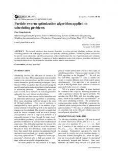
For this, we use the standard sequential binomial lattice algorithm. Table 5.11 presents option values computed by binomial lattice and our sequential PSO-based algorithm; also presented in this table are the execution time for both methods. Note that the number of iterations of our PSO-based algorithm is equivalent to time steps of binomial lattice. The option value is computed for S = 21, K = 25, σ = 0.3, N = 20 , r = 0.05. Similarly, Figure 5.1 presents execution time of our sequential and binomial lattice


σ 0.3 0.4 0.5 0.75 0.3 0.4 0.5 1 0.3 0.4 0.5

time 0.33 0.35 0.37 0.2 0.61 0.1 0.74 0.73 0.82

PSO-value 4.61 4.84 5.04 4.77 5.34 5.53 5.36 5.8 6.2

42 BSM-value 5.04 5.53 6.07 5.56 6.19 6.88 6.03 6.78 7.59


T 0.5

σ 0.3 0.4 0.5 0.75 0.3 0.4 0.5 1 0.3 0.4 0.5

time 0.12 0.33 0.37 0.48 0.29 0.48 0.79 0.25 0.44

PSO-value 0.7 0.78 1.41 0.9 1.17 1.44 1.22 1.53 1.88

BSM-value 0.75 1.31 1.9 1.2 1.93 2.49 1.63 2.49 3.37


model. We observe that binomial lattice works faster than our sequential algorithm. Note that in the PSO algorithm, we use random number generators for the parameters r1 and r2 in Equation 4.3 for each of the N particles at each iteration. During each iteration, to avoid duplication we discard some of the random numbers generated among particles and regenerate more random numbers. This adds to overhead and the cost of the overhead in PSO in presented in the table 5.11 as well. For future work, we plan to use parallel pseudo-number generator to reduce this overhead cost.


T 0.5 0.75 1

σ 0.5 0.5 0.4

time 0.34 0.29 0.63

PSO-value 6.85 7.49 7.99

43

BSM-value 6.6 7.31 7.24

Itr 10000 10000 10000

Table 5.7: Call option value for S = 25, K = 20, N =40

T 1 1 1 1

σ 0.4 0.4 0.5 0.5

time 0.27 0.22 0.52 0.47

PSO-value 1.62 1.66 1.97 2.19

BSM-value 2.49 2.49 3.37 3.37

Itr 1000 10000 1000 10000

Table 5.8: Call option value for S = 22, and K = 26, N = 40

T 0.5 0.75 1

σ rand rand rand

value 3.9 5.2 6.2

time 0.3 0.14 0.8

Table 5.9: Call option value with random volatility for S = 21, K = 23

T 0.5 0.75 1

σ rand rand rand

value 1.42 2.17 3.00

time 0.5 0.67 0.8

Table 5.10: Call option value with random volatility for S = 21, K = 23


Algorithm time step/iterations value Exec. time PSO overhead Binomial 1000 5.90 0.0271 PSO-based 1000 5.1 0.1819 0.0688 Binomial 10000 5.90 2.4724 PSO-based 10000 5.4 6.71 3.1471

Table 5.11: Binomial lattice vs sequential PSO-based algorithm

Figure 5.1: Binomial lattice vs sequential PSO-based algorithm

44


5.2

45

Parallel PSO Algorithm

We have implemented and tested our parallel algorithm on Helium cluster, a cluster of Linux servers available at the University of Manitoba, Department of Computer Science. The cluster consists of one head node and five computing nodes. The head node is a Sun Fire X4200 machine. Its configuration is as follows: Processor: one Dual-Core AMD Opteron 252 2.6GHz Memory: 2.0GB Cache size : 1MB/each core OS: CentOS 5 The five computing nodes are named as helium-01, helium-02, . . ., helium-05. Each is a Sun Fire X4600 machine. Its configuration is as follows. Processor: eight Dual-Core AMD Opteron 885 2.6GHz (totally 16 cores each node) Memory: 32GB Cache size : 1 MB L2/each core OS: CentOS 5 CPU Interconnect: HyperTransport speed (1GHz, 8GB/s) The parallel algorithm is implemented on a cluster of four nodes (H = 4) with eight dual-core processors, 64 homogeneous multi-core processors in total. We test

Chapter 5: Experimental Results and Discussion T 0.5 0.5 0.5 0.75 0.75 0.75 1 1 1

σ 0.3 0.4 0.5 0.3 0.4 0.5 0.3 0.4 0.5

PSO-value 4.47 4.71 5.01 4.69 5.03 5.21 5.01 5.87 5.94

time 0.16 0.32 0.22 0.20 0.35 0.19 0.15 0.92 0.19

46 BSM-value 4.96 5.42 5.94 5.45 6.05 6.71 5.9 6.61 7.38

Table 5.12: Parallel PSO-based call option value for S = 25 and K = 21 the algorithm on a shared memory address space, distributed message passing environment and hybrid (shared address space and distributed memory) environment. First, we check the accuracy of our parallel algorithm results. In tables 5.12 and 5.13, we present option value computed using our parallel algorithm implemented on a shared memory address space (8 dual-core or 16 processors). We compare our pricing results with Black-Scholes-Merton model for different time period and volatility for two cases (S = 25, K = 21, r = 0.05, N = 20 and Itr = 1000) and (S = 21, K = 25, r = 0.05, N = 20 and Itr = 1000). The result shows that the option value computed from our parallel algorithm is comparable with Black-Scholes-Merton model in most of the cases. We discuss Figure 5.2 observations in terms of speedup in subsection 5.2.1. Figures 5.3, 5.4, and 5.5 show the execution time results with respect to number of particles for three different number of iterations, 1000, 10, 000 and 30, 000. These results show that as the number of iterations increases, the sequential PSO algorithm’s performance degrades.


47

Figure 5.2: Parallel binomial vs parallel PSO-based algorithm

4.5

Serial 4

3.5 Hybrid-4 3

Hybrid-3

2.5

Execution Time in secs

2 Hybrid-2

1.5

1

OpenMP

0.5 MPI 0 16

20

24

30

36

42

48

52

58

64

Number of Particles

Figure 5.3: Execution Time for Itr = 1000


48

25

MPI

20 OpenMP

15 Hybrid-2

Execution Time in secs 10

Hybrid-3

Hybrid-4 5

Serial 0 16

20

24

30

36

42

48

52

58

64

Number of Particles

Figure 5.4: Execution Time for Itr = 10000 200 MPI 180

160 OpenMP 140

120 Hybrid -2

Execution 100 Time in secs 80

Hybrid -3

60

Hybrid -4

40

20 Serial 0 16

20

24

30

36

42

48

52

58

64

Number of particles

Figure 5.5: Execution Time for Itr = 30000


49

40 Total Execution Time 35

30 Communication Cost 25

20

Barrier Cost

Execution Time in secs 15

Computation

10

5 Context switching 0 16

20

24

30

36

42

48

52

58

64

Number of particles

Figure 5.6: Execution Time Analysis in MPI for Itr = 30000

90

Total Execution Time

80

70

Communication Cost

60

50


Barrier Cost

40

30 Computation 20


20

24

30

36

42

48

52

58

64

Number of particles

Figure 5.7: Execution Time Analysis in openMP for Itr = 30000


50

45


40

35

Communication Cost

30

25

Execution 20 Time in secs

Barrier Cost

15 Computation 10


20

24

30

36

42

48

52

58

64

Number of particles

Figure 5.8: Execution Time Analysis in Hybrid-2 for Itr = 30000

Figure 5.9: Execution Time Analysis in Hybrid-3 for Itr = 30000

Chapter 5: Experimental Results and Discussion T 0.5 0.5 0.5 0.75 0.75 0.75 1 1 1

σ 0.3 0.4 0.5 0.3 0.4 0.5 0.3 0.4 0.5

PSO-value 0.49 0.64 0.96 0.66 0.93 1.37 1.22 1.43 1.84

51

time 0.22 0.13 0.17 0.49 0.5 0.34 0.93 0.43 0.48

BSM-value 0.68 1.21 1.77 1.1 1.8 2.51 1.5 2.33 3.16

Table 5.13: Parallel PSO-based call option value for S = 21 and K = 25 10


9

8

7

Communication Cost

6

5


Barrier Cost

4

3 Computation 2

1

0

Context switching 16

20

24

30

36

42

48

52

58

64

Number of particles

Figure 5.10: Execution Time Analysis in Hybrid-4 for Itr = 30000 Figures 5.6-5.10 and Tables 5.14-5.18 present detailed costs (computation, communication, barrier, and context switching) of our parallel algorithm on the three implementations for 30, 000 iterations. From these figures and tables, we can see

Chapter 5: Experimental Results and Discussion N 16 20 24 30 36 42 48 52 58 64

Total 9.63706 13.138794 14.624433 17.165423 20.245002 25.337552 25.6659 27.322814 29.599099 35.04949

Communication 3.34837 3.952786 4.398757 6.339603 7.134161 7.534619 9.341526 9.977233 10.611122 13.366944

Barrier 3.215363 6.063423 7.07041 7.716524 10.003356 14.819025 13.210293 14.249422 15.850164 18.465184

52 Computation 3.073327 3.122585 3.155266 3.109296 3.107485 2.983908 3.114081 3.096159 3.137813 3.217362

Context Switching 0 0 0 0 0 0 0 0 0 0

Table 5.14: MPI Execution Time (in secs) Analysis N 16 20 24 30 36 42 48 52 58 64

Total 3.916972 15.527018 31.261782 37.581378 44.371843 60.587454 68.851265 68.452747 78.460243 84.969199

Communication 0 0 0 0 0 0 0 0 0 0

Barrier 0.524821 3.782566 3.85937 3.891961 3.950918 4.448343 4.690366 4.82593 5.41393 5.826544

Computation 3.40686 3.60123 3.76315 4.140686 4.23616 4.67812 4.94731 5.3686 5.740612 5.99621

Context Switching 0 8.143222 23.639262 29.548731 36.184765 51.460991 59.213589 58.258217 67.305701 73.146445

Table 5.15: OpenMP Execution Time (in secs) Analysis that context switching and communication cost is reduced in hybrid implementation. Also, as number of particles increases, in each hybrid model (hybrid-2, hybrid-3, and hybrid-4) , the communication cost almost remain similar. However, as the number of particles increase the barrier cost increases. This is due to the synchronization barrier that is needed when the central processor computes the global result. To overcome the barrier costs, as future work, a parallel asynchronous PSO based option pricing


Total 5.495242 5.70468 5.900409 6.209401 14.518815 26.534724 31.068775 34.701664 36.07178 38.567129

Communication 0.523812 0.523825 0.524181 0.538388 0.560297 0.580799 0.597944 0.605067 0.594344 0.609588

Barrier 1.224079 1.333155 1.345766 1.504567 3.803194 7.341777 8.601333 9.720564 10.46071 11.686713

53 Computation 3.747351 3.8477 4.030462 4.166446 4.291724 4.847948 5.218298 5.393723 5.424626 5.527228

Context Switching 0 0 0 0 5.8636 13.7642 16.6512 18.98231 19.5921 20.7436

Table 5.16: Hybrid-2 Execution Time Analysis N 16 20 24 30 36 42 48 52 58 64

Total 5.8553 5.9169 5.6446 6.6581 6.0665 7.3985 7.7048 17.6403 19.9456 21.1962

Communication 0.629113 0.633984 0.619135 0.623361 0.619495 0.623361 0.63327 0.659233 0.658865 0.665801

Barrier 1.10415 1.285973 1.610317 1.876876 2.03861 2.22361 2.62652 4.912761 5.748794 6.382889

Computation 4.122037 3.996943 3.415148 4.157863 3.408395 4.551529 4.44501 5.872006 7.320341 6.29561

Context Switching 0 0 0 0 0 0 0 7.1963 7.6176 9.2519

Table 5.17: Hybrid-3 Execution Time Analysis algorithm can be explored.

5.2.1

Parallel Algorithms’ Speedup

Table 5.19 shows the execution time for parallel binomial lattice algorithm and PSO algorithm on a distributed memory architecture. We notice that the PSO paral-


Total 6.705214 6.510182 6.878896 7.063141 7.32036 7.493296 7.78891 7.86331 8.113185 8.729292

Communication 0.669102 0.643899 0.640903 0.635949 0.643695 0.629022 0.653641 0.636495 0.643652 0.643695

Barrier 1.67314 1.865976 1.82014 1.902493 2.057069 2.124872 2.28721 2.33722 2.514872 2.684872

Computation 4.362972 4.000307 4.417853 4.524699 4.619596 4.739402 4.848059 4.889595 4.954661 5.400725

54 Context Switching 0 0 0 0 0 0 0 0 0 0

Table 5.18: Hybrid-4 Execution Time Analysis N 16 20 24 30 36 42 48 52 58 64

parallel binomial parallel PSO-based algorithm Itr 0.202 0.2959 1000 0.194 0.4187 1000 0.205 0.5218 1000 0.221 0.6445 1000 0.229 0.7881 1000 0.233 0.7917 1000 0.252 0.9814 1000 0.269 1.0997 1000 0.307 1.1639 1000 0.431 1.3286 1000

Table 5.19: Parallel execution time in a distributed memory architecture lel execution time exceeds that of binomial lattice method. This is mainly due to (i) overhead caused by PSO computations for particle position update, and (ii) random number generation (mentioned earlier). These points and the communication bottleneck on distributed memory machines motivated us to consider the shared address space and hybrid architectures. In the tables 5.20-5.22, hybrid-H represents H nodes with 8 dual-cores or 16 pro-


openmp 0.072 0.2338 0.2871 0.3747 0.4042 0.5229 0.5449 0.6121 0.662 0.7169

hybrid-2 0.1079 0.1355 0.1287 0.2034 0.3265 0.353 0.4167 0.4374 0.4719 0.513

hybrid-3 0.1026 0.1093 0.1102 0.139 0.15 0.1583 0.1703 0.3289 0.3682 0.3818

55 hybrid-4 0.1292 0.132 0.1344 0.1362 0.1495 0.1712 0.1836 0.1904 0.218 0.417

Itr 1000 1000 1000 1000 1000 1000 1000 1000 1000 1000

Table 5.20: Parallel execution time in shared memory and hybrid architecture cessors per node. Table 5.20 shows the execution time on shared memory and hybrid architectures. The parallel PSO algorithm on the hybrid architecture performs better than the shared memory architecture as we increase the number of particles. In shared memory architecture, due to context switching the execution time is higher as we increase the number of particles. Tables 5.21 and 5.22 present speedup results of parallel PSO-based option pricing algorithm on shared and hybrid architectures for larger number of iterations. The speedup [Grama et al., 2003] is defined as

T1 TP

where T1 is the execution time of the

sequential PSO algorithm on one processor and TP is the execution time for parallel PSO algorithm on P processors. First, let us consider the shared memory results. We observe that for 16 particles the speedup for 30000 iterations is higher than that of 10000 iterations. As the number of particles increases, in both tables we notice that the shared memory speedup results is significantly lower. The reason for this is as follows. The implementation of the


56

PSO algorithm is performed on 16 processors. In the case of N = 16, each particle, regarded as a thread, is allocated to one processor. When N > 16, say N = 36, each processor is allocated two particles with the exception of four processors allocated with three particles. In this case, the work is not well balanced. Also, in shared memory machines, the processors context switch between threads, which creates additional overhead. Next, we compare the hybrid implementation results. Recall that hybrid-H represents H nodes with P processors. In our cluster, there are 16 processors per node. Hybrid-2 refers to 2 nodes with 32 processors, hybrid-3 refers to 3 nodes with 48 processors and hybrid-4 refers to 4 nodes with 64 processors. Also, recall that there is shared memory within each node and nodes communicate through message passing. Initially, we distribute N/H particles among the H nodes. Among all the three hybrid cases, hybrid-4 produces better speedup results for both 10, 000 and 30, 000 iterations. We explain this as follows. When N = 64, each particle is allocated to each of the 64 processors in hybrid-4 cluster. Since shared memory performs better if there is one to one mapping of processors to threads as explained above for the shared memory results, the results for N = P produces the desired speedup results for hybrid-4 cluster. When N < 64, some of the processors in hybrid-4 cluster are idle. For example, when N = 48, each node is allocated 48/4 = 12 particles per node. In this case, four processors per node are idle. When N = 16, 16/4 = 4 particles are allocated per node, with 12 processors idle per node. As we increase N, we are able to reduce number of idle processors through load balancing. Therefore, we notice increase in the speedup.


57

We can extend this observation to the other hybrid-H cases. When N = 48, hybrid3 performs well. Again, this is due to the one to one mapping between particles and processors. In hybrid-3, unlike hybrid-4, some processors may be idle or may have more particles per processor. For example, in the case when N = 36, 36/3 = 12 particles are allocated to each node. In this case, four processors/node are idle. As explained in the hybrid-4 case, this load imbalance creates poor speedup. We can see from the tables that for all values of N < 48, the speedup with hybrid-3 is not comparable to N = 48. Now, when N = 64 (N > 48), 64/3 = 21 particles are allocated per node. Each particle is scheduled to each of the 16 processors/node with five processors in each node allocated one extra particle. As mentioned in the shared memory results there is more work for some processors (unbalanced workload) and therefore the speedup results fall below that of N = 48. Note that, in the parallel PSO algorithm for the hybrid case, particles within a node compute independently of the other particles in other nodes until the calculation of global best. The master processor for each node, masterL , gathers the global local best results from each of its assigned particles, and sends the result to the central processor, masterG . At the end of each iteration, a comparison among the local best values (determined by masterL in each node) are done by masterG . Since the computations within a node are local, the amount of communication to the master, masterG is very low. That is, each node communicates its local best among its assigned particles and masterL sends one best value to the masterG . In general, for hybrid-H, there is basically 2*(H-1) amount of communication between the nodes and masterG . Therefore, for I iterations, 2*(H-1)*I communication is performed. This


openmp 5.63 1.95 1.93 1.75 1.71 1.62 1.51 1.55 1.54 1.53

hybrid-2 5.13 5.45 6.33 7.44 3.33 3.06 3.28 3.07 2.98 3.22

hybrid-3 4.73 5.45 6.49 7.75 8.43 10.08 11.25 4.01 4.38 4.77

58 hybrid-4 4.42 4.94 5.75 6.98 7.78 8.80 9.66 9.68 9.28 8.09

Itr 10000 10000 10000 10000 10000 10000 10000 10000 10000 10000

Table 5.21: Parallel PSO-based algorithm speedup in shared and hybrid architecture does not seem to cause a performance degradation issue as can be seen from N = P cases in each of the hybrid-H results. We conclude from these results that, for a shared memory architecture or a hybrid architecture, a one to one mapping of particles to processors is recommended for performance speedup. Load imbalance and idle processors degrade the performance. A hybrid architecture reduces the communication overhead cost that is incurred in a pure distributed memory architecture. It is also best if we reduce the communication as much as possible.


N 16 20 24 30 36 42 48 52 58 64

openmp 11.47 3.63 2.16 2.24 2.27 1.94 1.95 2.12 2.07 2.11

hybrid-2 8.17 9.87 11.44 13.53 6.95 4.43 4.32 4.19 4.51 4.64

hybrid-3 7.67 9.52 11.96 12.62 16.63 15.90 17.44 8.25 8.15 8.45

59

hybrid-4 6.70 8.65 9.82 11.89 13.78 15.70 17.25 18.50 20.05 20.51

Itr 30000 30000 30000 30000 30000 30000 30000 30000 30000 30000

Table 5.22: Parallel PSO-based algorithm speedup in shared and hybrid architecture

Chapter 6 Conclusion and Future work The major contribution from this work is the conceptualization of PSO for the option pricing problem, and design of sequential and parallel algorithms from fundamental principles of PSO. To the best of our knowledge, this is the first attempt to use Particle Swarm Optimization for an American option pricing problem. We studied both velocity equations (Shi and Eberhart (Equation 3.6) and Clerc and Kennedy (Equation 3.8)) to incorporate volatilities for option pricing, and chose Shi and Eberhart velocity equation (Equation 3.6) to implement. In both velocity equations, we consider constant and dynamic volatility. The random part of ω acts as volatility of the underlying asset in Shi and Eberhart velocity equation. The particles collaborate in achieving the objective of exercising a given option at the best possible time that gives optimal option price results. The collaboration is achieved through local best (for a particle) and global best (for swarm) concepts. The discounting feature for an option is carefully employed for the local and global best computation to achieve the objective.

60

Chapter 6: Conclusion and Future work

61

We have studied the performance evaluation of PSO-based sequential and parallel option pricing algorithms. First, we tested the accuracy of the algorithm against Black-Scholes-Merton model for various volatility and contract period. The PSO algorithm converges to Black-Scholes-Merton model when the number of iterations increases together with the number of particles. The execution time of the sequential PSO algorithm is slightly higher in comparison to the binomial lattice algorithm. This we attribute to the overall cost of generating many random numbers by the particles at each iteration. Since it is very important and critical to lock-in the profit making opportunities in the real market, we have also designed and developed a parallel algorithm to expedite the computing process. The parallel PSO-based algorithm is tested on three different architectures: distributed, shared, and hybrid using up to 64 processors. We compare speedup of our parallel algorithm against parallel binomial lattice. The speedup results show that the parallel PSO-based algorithm has better speedup than parallel binomial lattice algorithm. We conclude that for a shared memory architecture or a hybrid architecture, as we increase the problem size for better accuracy, it is advisable to use more number of processors in order to maintain a level of speedup. In other words, one-to-one mapping of particles to processors is desirable. We also noticed that hybrid architecture helps to reduce the communication overhead cost that incurs in distributed architecture. The speedup of our algorithm increases for larger number of iterations. The speedup is 20 in hybrid architecture using four computing nodes. We observe that load imbalance and idle processors degrade the performance; as expected. To circumvent this problem, an asynchronous parallel algorithm can be

Chapter 6: Conclusion and Future work

62

designed. Further improvement in our algorithm is possible by dynamically changing the PSO parametric conditions, finance parameters, and termination condition for the algorithm, which we leave as future work. Along with these, the PSO-based option pricing algorithms can be also extend for complex options.

Bibliography S. Barua, R. K.Thulasiram, and P. Thulasiraman. High performance computing for a financial application using fast Fourier transform. In Proceedings of the European Parallel Computing Conference, (EuroPar 2005), volume 3648, pages 1246–1253, Lisbon, Portugal, 2005. M. A. J. Bharadia, N. Christofides, and G. R. Salkin. Computing the Black-Scholes implied volatility: Generalization of a simple formula. Advances in Futures and Options Research, 8:15–29, 1995. M. A. J. Bharadia, N. Christofides, and G. R. Salkin. A quadratic method for the calculation of implied volatility using the Garman-Kohlhagen model. Financial Analysts Journal, 52:61–64, 1996. B. Birge. PSOt-a particle swarm optimization toolbox for use with Matlab. In Proceedings of the 2003 IEEE swarm intelligence symposium, pages 182–186, December 2003. F. S. Black and M. S. Scholes. The pricing of options and corporate liabilities. Journal of Political Economy, 81:637–654, January 1973.

63

Bibliography

64

P. Boyle. Options: A Monte Carlo approach. Journal of Financial Economics, 4: 223–238, 1977. A. Brabazon and M. O’Neil. Biologically Inspired Algorithms for Financial Modelling (Natural Computing Series). Springer-Verlag, 2006. B. Bullnheimer, R. F. Hartl, and C. Strauss. An improved ant system algorithm for the vehicle routing problem. In Annals of Operations Research, volume 89, pages 319–328, 1999. G. D. Caro, F. Ducatelle, and L. M. Gambardella. AntHocNet: An adaptive nature inspired algorithm for routing in mobile ad hoc networks. European Transactions on Telecommunications (Special Issue on Self-Organization in Mobile Networking), 16:443–455, 2005. P. Carr and D. B. Madan. Option valuation using the fast Fourier transform. The Journal of Computational Finance, 2(4):61–73, 1999. P. Chalasani, S. Jha, F. Egriboyun, and A. Varikooty. A refined binomial lattice for pricing American Asian options. Review of Derivatives Research, 3:85–105, January 1999. D. M. Chance. A generalized simple formula to compute the implied volatility. The Financial Review, 3:859–867, 1996. S.-H. Chen, W.-C. Lee, and C.-H. Yeh. Hedging derivative securities with genetic programming. International Journal of Intelligent Systems in Accounting, Finance and Management, 8:237–251, 1999.

Bibliography

65

Y. Chen, B. Yang, and J. Dong. Evolving flexible neural networks using ant programming and PSO algorithm. LNCS 3173, pages 211–216, 2004. Y. Chen, B. Yang, and J. Dong. Time series prediction using a local linear wavelet neural network. Neurocomputing, pages 449–465, 2005. Y. Chen, B. Yang, and J. Dong. Time-series prediction using a local linear wavelet neural network. Neurocomputing, 69:449–465, 2006. N. K. Chidambaran, C. W. J. Lee, and J. R. Trigueros. Option pricing via genetic programming. In Computational Finance-Proceedings of the Sixth International Conference, Leonard N. Stem School of Business, pages 583–598, January 1999. M. Clerc and J. Kennedy. The particle swarm-explosion, stability, and convergence in a multidimensional complex space. IEEE Transactions on Evolutionary Computation, 6:62–73, February 2002. J. C. Cox, S. A. Ross, and M. Rubinstein. Options pricing: A simplified approach. Journal of Financial Economics, 7:229–263, 1979. M. Dorigo, V. Maniezzo, and A. Colorni. Ant system–optimization by a colony of cooperating agents. IEEE Transactions on Systems, Man and Cybernetics, 26: 29–41, February 1996. R. Eberhart and Y. Shi. Tracking and optimizing dynamic systems with particle swarms. In Proceedings IEEE World Congresss on Evolutionary Computation, pages 94–97, Seoul, Korea, 2001.

Bibliography

66

A. Grama, A. Gupta, G. Karypis, and V. Kumar. Introduction to Parallel Computing. Pearson Education Limited, 2003. ISBN 02016485652. K. Huang and R. K. Thulasiram. Parallel algorithm for pricing American Asian options with multi-dimensional assets. In Proc. (CD-RoM) 19th Intl. Symp. High Performance Computing Systems and Applications (HPCS), pages 177–185, Guelph, ON, Canada, May 2005. J. Hull. Options, Futures, and other Derivative Securities. Prentice Hall, 7 edition, May 2008. J. M. Hutchinson, A. W. Lo, and T. Poggio. A nonparametric approach to pricing and hedging derivative securities via learning networks. Journal of Finance, 49: 851–889, 1994. G. K. Jha, S. Kumar, H. Prasain, P. Thulasiraman, and R. K. Thulasiram. Option pricing using particle swarm optimization. In Proceedings of the 2009 C* conference on computer science and software engineering (C3S2E) conference, pages 267–272, May 2009a. G. K. Jha, P. Thulasiraman, and R. K. Thulasiram. PSO based neural network for time series forecasting. In Proceedings of IEEE International Joint Conference on Neural Networks, pages 1422–1427, June 2009b. C. Keber. Genetically derived approximations for determining the implied volatility. OR Specktrum, 21:205–238, 1999.

Bibliography

67

C. Keber and M. G. Schuster. Generalized ant programming in option pricing: determining implied volatilities based on American put options. In IEEE Proceedings of Computational Intelligence in Financial Engineering, pages 123–130, December 2003. J. Kennedy and R. Eberhart. Particle swarm optimization. In Proceedings of the IEEE International Conference on Neural Networks, pages 1942–1958, March 1995. B. Koh-II, A. D. George, R. T. Haftka, and B. J. Fregly. Parallel asynchronous particle swarm optimization. International Journal For Numerical Methods in Engineering, 67:578–595, January 2006. S. Kumar, R. K. Thulasiram, and P. Thulasiraman. A bioinspired algorithm to price options. In ACM Proc. of the C* Conference on Computer Science and Software Engienering, pages 11–22, Montreal, May 2008. S. Kumar, R. K. Thulasiram, and P. Thulasiraman. ACO for Option Pricing, volume 2 of SCI 185, chapter 4, pages 51–73. Springer-Verlag, 2009. S. Lee, J. Lee, D. Shim, and M. Jeon. Binary particle swarm optimization for balckscholes option pricing. LNCS, 4692:85–92, 2007. J. Li, D. Wang, S. Chi, and X. Hu. An efficient fine-grained parallel particle swarm optimization method based on GPU-acceleration. International Journal of Innovation Comupting, Information and Control, 3(B(6)):1707–1714, December 2007. V. Maniezzo and A. Colorni. The ant system applied to the quadratic assignment problem. Knowledge and Data Engineering, 11(5):769–778, 1999.

Bibliography

68

R. C. Merton. Theory of rational option pricing. Bell Journal of Economics and Management Science, 4:141–183, 1973. J. Nenortait˙e. A particle swarm optimization approach in the construction of decisionmaking model. Information Technology and Control, 36:449–465, 2007. S. Rahmayil, I. Shiller, and R. K. Thulasiram. Different estimators of the underlying asset’s volatility and option pricing errors: parallel Monte-Carlo simulation. In Proceedings of the International Conference on Computational Finance and its Applications (ICCFA), pages 121–131, Bologna, Italy, 2004. J. Schutte, B.J.Fregly, R. Haftka, and A.D.George. A parallel particle swarm optimizer. International Journal For Numerical Methods in Engineering, 61:2296–2315, October 2004. Y. Shi and R. Eberhart. A modified particle swarm optimizer. In Proceedings IEEE World Congresss on Evolutionary Computation, pages 69–73, Archorage, AK, USA, May 1998. R. K. Thulasiram and P. Thulasiraman. Performance evaluation of a multithreaded fast Fourier transform algorithm for derivative pricing. The Journal of Supercomputing, 26(1):43–58, August 2003. R. K. Thulasiram, L. Litov, H. Nojumi, C. Downing, and G. Gao. Multithreaded algorithms for pricing a class of complex options. In Proceedings (CD-RoM) of the IEEE/ACM International Parallel and Distribued Processing Symposium (IPDPS), San Francisco, CA, 2001.

Bibliography

69

I. C. Trelea. The particle swarm optimization algorithm: convergence analysis and parameter selection. Information Processing Letters, 85:317–325, March 2003. G. Venter and J. Sobieszczanski-Sobieski. A parallel particle swarm optimization algorithm accelerated by asynchronous evaluations. Journal of Aerospace Computing, Information, and Communication, 3(3):123–137, March 2006. J. Wang, E. Osagie, P. Thulasiraman, and R. K.Thulasiram. Hopnet: A hybrid ant colony optimization routing algorithm for mobile ad hoc network. Ad Hoc Networks, 7:690–705, 2009. H. F. Wedde, M. Farooq, T. Pannenbaecker, B. Vogel, C. Mueller, J. Meth, and R. Jeruschkat. BeeAdHOC: An energy efficient routing algorithm for mobile ad hoc networks inspired by bee behavior. In Proceedings of Genetic and Evolutionary Computation Conference, pages 153–160, Washington, DC, June 2005. Z. Yin, A. Brabazon, and C. O’Sullivan. Adaptive genetic programming for option pricing. In Proceedings of the 2007 conference companion on Genetic and evolutionary computation (GECCO), pages 2588–2594, London, England, UK, 2007.