Patterns in Large Datasets. Qinghua Zou, Wesley Chu, David Johnson, Henry Chiu. Computer Science Department. University of California â Los Angele.
A Pattern Decomposition (PD) Algorithm for Finding All Frequent Patterns in Large Datasets Qinghua Zou, Wesley Chu, David Johnson, Henry Chiu Computer Science Department University of California – Los Angele Abstract Efficient algorithms to mine frequent patterns are crucial to many tasks in data mining. Since the Apriori algorithm was proposed in 1994, there have been several methods proposed to improve its performance. However, most still adopt its candidate set generation-and-test approach. We propose a pattern decomposition (PD) algorithm that can significantly reduce the size of the dataset on each pass making it more efficient to mine frequent patterns in a large dataset. The proposed algorithm avoids the costly process of candidate set generation and saves time by reducing dataset. Our empirical evaluation shows that the algorithm outperforms Apriori by one order of magnitude and is faster than FP-tree. Further, PD is more scalable than both Apriori and FP-tree.
1. Introduction A fundamental process in data mining is finding frequent patterns in a given dataset. Finding frequent patterns facilitates essential tasks such as discovering association relationships between items, correlation, and sequential patterns [7]. A significant problem with mining frequent larger patterns is that as the length of the pattern increases, the number of potential patterns grows at a combinatorial rate. Several different algorithms have been proposed to efficiently find all frequent patterns in a dataset [1,5,6,7]. Other algorithms output only maximal frequent sets, thus minimizing the number of potential patterns [2, 3, 4]. Max-Miner [2] uses a heuristic bottom-up search to identify frequent patterns as early as possible. PincerSearch [4] uses a bottom-up search along with top-down pruning. Even though performance improvements may be substantial, maximal frequent sets have limited use in association rule mining. A complete set of rules cannot be extracted without support information of the subsets of those maximal frequent sets. FP-tree-based mining [9] is a different approach in that it first builds up an optimized data representation (FP-tree) from the dataset. All mining tasks are then performed on the FP-tree rather than on the dataset.
Proceedings of the 2001 IEEE International Conference on Data Mining (ICDM’01) 0-7695-1119-8/01 $17.00 © 2001 IEEE
In this paper we propose an innovative algorithm called Pattern Decomposition (PD) that generates all frequent sets. The algorithm provides increased performance by reducing the dataset during each pass. The dataset is reduced by splitting transactions and combining similar transactions together, thus decreasing counting time and improving performance. In addition, the algorithm does not need to generate candidate sets; all subsets of any transaction in the reduced dataset are frequent thus should be counted. Intuitively, a transaction that contains infrequent itemsets can be decomposed to smaller itemsets if together they do not meet the minimum support threshold. Frequently, after splitting all the transactions in the dataset many itemsets are identical and can be combined, thus reducing the size of the dataset.
2. The Method The PD algorithm shrinks dataset each time when infrequent itemsets are discovered. More specifically, it finds frequent sets by employing a bottom-up search. For a given transaction dataset D1, the first pass has two phrases: 1) the algorithm counts for item occurrences to determine the frequent 1-itemsets L1 and the infrequent 1itemsets ~L1; 2) we decompose D1 to D2 such that D2 contains no items in ~L1. Similarly, in a subsequent pass, say pass k, frequent itemsets Lk and ~Lk are generated by counting for all k-itemsets in Dk. Then, Dk+1 is generated by decomposing Dk using ~Lk such that Dk+1 contains no itemsets in ~Lk. Now let us illustrate the complete process for mining frequent patterns. In Figure 1, we show how PD is used to find all frequent patterns in a dataset. Suppose the original data set is D1 and minimal support is 2. We first count the support of all items in D1 to determine L1 and ~L1. In this case, frequent 1-itemset L1={a,b,c,d,e} and infrequent 1-itemset ~L1={f,g,h,k}. Then we decompose each pattern in D1 using ~L1 to get D2. In the second pass, we generate and count all 2-item sets contained in D2 to determine L2 and ~ L2, as shown in the figure. Then we decompose each pattern in D2 to get D3. This continues until we determine D5 from D4, which is the empty set and we terminate. The final result is the union of all frequent sets L1 through L4.
The example illustrates three ways to reduce the dataset as denoted by α, β, δ in Figure 1. In α, when patterns D1 D2 1:a b c d e f: 1 f 1:a b c d e: 1 after decomposition 2:a b c g: 1 g 2:a b c: 2 yield the same 3:a b d h: 1 h 3:a b d: 1 itemset, we combine 4:b c d e k: 1 k 4:b c d e: 1 them by summing 5:a b c: 1 α L ~L2 their occurrence. 2 L1 ~L1 IS Occ IS Occ Here, abcg and abc IS Occ IS Occ {ab} 4 {ae} 1 reduce to abc. Since {a} 4 {f} 1 {ac} 3 both their {b} 5 {g} 1 {ad} 2 occurrences are 1, the {c} 4 {h} 1 {bc} 4 final pattern is abc:2 {d} 3 {k} 1 {bd} 3 in D2. {e} 2 {be} 2 In β, we remove {cd} 2 D3 patterns if their sizes {ce} 2 1: abcd, bcde: 1 {de} 2 are smaller than the 2: a b c: 2 3: a b d: β 1 δ D4 required size of the 1: b c d e: 2 4: b c d e: 1 next dataset. Here, ~L4 L4 L3 ~L3 patterns abc and abd IS Occ IS Occ IS Occ IS Occ with sizes of 3 cannot {abc} 3 {acd} 1 {bcde} 2 be in D4 and are {abd} 2 deleted. {bcd} 2 D5= Φ In δ, when a part of {bce} 2 a given pattern has {bde} 2 Figure 1. Pattern {cde} 2 Decomposition Example the same itemset with another pattern after decomposition, we combine them by summing their occurrence. Here, bcde is the itemset of pattern 4 and part of pattern 1’s itemset after decomposition, so the final pattern is bcde:2 in D4. One simple way to decompose the itemset s by an infrequent k-item set t, as explained in [4], is to replace s by k itemsets, each obtained by removing a single item in t from s. For example, for s = abcdefgh and t = aef, we decompose s by removing a, e, f respectively to obtain {bcdefgh, abcdfgh, abcdegh}. We call this method simple-split. When the infrequent sets are large, simplesplit is not efficient. Thus PD needs Quick-split to decompose a pattern. [8]
3. Performance Study We compare PD with Apriori and FP-tree since the former is widely cited and the latter claims the best performance in the literature. The test data sets were generated in the same fashion as the IBM Quest project [1]. We used two data sets T10.I4.D100K and T25.I10.D100K. For the comparison of PD with FP-tree, since PD was written in Java and FP-tree in C++ and we don’t have time to implement PD in C++, their results are adjusted by a coefficient about 10. Our study shows that PD is about 30 times faster than Apriori with minimal support at 2% and about 10 times faster than Apriori at 0.25%. The execution time for
Proceedings of the 2001 IEEE International Conference on Data Mining (ICDM’01) 0-7695-1119-8/01 $17.00 © 2001 IEEE
Apriori linearly increases with the number of transactions from 50K to 250K. Better than that, the execution time for PD does not necessarily increase as the number of transactions increases. Both FP-tree and PD have better performance than Apriori. FP-tree takes substantially more time than PD does when minimum support in the range from 0.5% to 2%. When minsup less than 0.5%, the number of frequent patterns increased quickly and thus the execution times are comparable. PD is about 9 times faster than FPtree with minimal support at 2% and the gap reduces to 2 times faster at 0.25%. When the number of transactions ranged from 60k-80k, both methods took almost constant time (most likely due to overhead). When we scaled up to 200K, FP-tree required more than 1884M of virtual memory and could not run on our machine while PD finished the computation within 64M main memory. For more details, interested readers please refer to [8].
4. Conclusion We propose a pattern decomposition (PD) algorithm to find frequent patterns. The algorithm significantly shrinks the dataset in each pass. It avoids the costly candidate set generation procedure and greatly saves counting time by using reduced datasets. Our experiments show that the PD algorithm has an order of magnitude improvement over the Apriori algorithm on standard test data and is faster than FP-tree.
References [1] R. Agrawal and R. Srikant. Fast algorithms for mining association rules. In VLDB'94, pp. 487-499. [2] R. J. Bayardo. Efficiently mining long patterns from databases. In SIGMOD'98, pp. 85-93. [3] Zaki, M. J.; Parthasarathy, S.; Ogihara, M.; and Li, W. 1997. New Algorithms for Fast Discovery of Association Rules. In Proc. of the Third Int’l Conf. on Knowledge Discovery in Databases and Data Mining, pp. 283-286. [4] Lin, D.-I and Kedem, Z. M. 1998. Pincer-Search: A New Algorithm for Discovering the Maximum Frequent Set. In Proc. of the Sixth European Conf. on Extending DatabaseTechnology. [5] Park, J. S.; Chen, M.-S.; and Yu, P. S. 1996. An Effective Hash Based Algorithm for Mining Association Rules. In Proc. of the 1995 ACM-SIGMOD Conf. on Management of Data, pp. 175-186. [6] Brin, S.; Motwani, R.; Ullman, J.; and Tsur, S. 1997. Dynamic Itemset Counting and Implication Rules for Market Basket Data. In Proc. of the 1997 ACM-SIGMOD Conf. On Management of Data, 255-264. [7] J. Han, J. Pei, and Y. Yin. Mining Frequent Patterns without Candidate Generation. Proc. 2000 ACM-SIGMOD Int. Conf. on Management of Data, Dallas, TX, May 2000. [8] Q. Zou, H. Chiu, W. W. Chu, D. Johnson. Pattern Decomposition Algorithm for Data Mining Frequent Patterns. Journal of Knowledge and Information Systems, 2002 (to appear).