2016 IEEE 55th Conference on Decision and Control (CDC) ARIA Resort & Casino December 12-14, 2016, Las Vegas, USA
A Physics-Based Control-Oriented Model for Compressor Mass Flow Rate Kang Song, Devesh Upadhyay, Harold Sun, Hui Xie, and Guoming Zhu
Abstract—In this paper, a control-oriented model for compressor mass flow rate is proposed. For this purpose, the compressor is approximated as an adiabatic nozzle with compressible fluid, driven by external work from the compressor wheel. The external work input is modeled using Euler’s turbomachinery equations, with the main flow losses estimated via a simple slip factor model. All other flow losses, that influence the mass flow, are lumped into the discharge coefficient as a function of turbocharger speed. Consequently, the mass flow rate is estimated based on mass conservation in a compact form. Only five parameters need to be identified with clear physical interpretations. Both steady-state and transient experimental test results confirm the validity of this model in terms of estimation accuracy and extrapolation capability, making it a promising candidate for control applications.
I. INTRODUCTION Modern boosted engines rely on a variety of configurations involving Turbochargers (TC) and Exhaust Gas Recirculation (EGR) [1]. Recent developments in this area have introduced advanced systems involving assisted boosted configurations such as E-Turbo [2] that allows improved control bandwidth but with added complexity. In order to achieve accurate air path control for such coupled systems, it is necessary to define the essential TC dynamics accurately. The compressor mass flow rate is one such crucial performance variable [3]. Typical control models treat the compressor mass flow rate as a plant output derived from the compressor power which is in turn derived using a variety of approaches. In [3, 4] the compressor power is treated as a first order internal state with a fixed time constant to maintain energy flow causality. Another popular approach is to use supplier provided compressor maps. However, inherent limitations of flow bench tests, such as steady flow [5] conditions and a lack of heat transfer effects from the turbine [6], limits the use of these maps over a wide operating regime [2]. To overcome some of these drawbacks, extensive research efforts have been made on control-oriented TC modeling in the past. As early as 1991, Jensen et al. reported the well-known JK model [7]. In their model, the compressor was treated like a pump with the flow rate coefficient Φ modeled as an inverse proportional function of a dimensionless head parameter ψ and the blade Mach number. Following this idea, a number of other models were proposed, e.g., by replacing Song and Xie are with Tianjin University, Tianjin, 300072, China. (e-mail:
[email protected],
[email protected]). Song is now a research scholar at Michigan State University, East Lansing, MI, 48824, USA. Upadhyay and Sun are with Ford Motor Company, Dearborn, MI, 48124, USA. (e-mail:
[email protected] and
[email protected]). Zhu is with Michigan State University, East Lansing, MI, 48824, USA. (e-mail:
[email protected], phone: (517)-884-1552, fax: (517)-884-1552). 978-1-5090-1837-6/16/$31.00 ©2016 IEEE
the inverse proportional function with an ellipse function [8], or by building a relationship between the compressor geometries and the JK model coefficients [9]. Other modeling solutions, that use the pressure ratio instead of ψ, were also investigated, in the form of parabolic function [10] or piece-wise functions [3]. To some extent, these models all follow the same underlying principle, i.e., to estimate the flow rate coefficient Φ, although the particular expressions used may vary slightly. Some black-box modeling methods, such as neural network [11] were also investigated, but later proved not a good solution for the estimation of mass flow rate [3]. These aforementioned models do use some physics, but the key relationship between the dimensionless head parameter and the mass flow rate was largely artificial, leading to a variety of model expressions where the compressor mass flow rate is captured numerically rather than physically. As a consequence, problems arise from model extrapolation. For example, the JK model is prone to abrupt changes in estimated mass flow rate. This happens once the denominator of the Φ function crosses zero at high mass flow rates or low pressure ratios, determined by the nature of inverse proportional function. To achieve better extrapolation, Leufven and Eriksson [12] proposed an elliptic function based piece-wise model, which can predict the mass flow rate over a larger range of pressure ratios. Several map extrapolation and interpolation algorithms were also proposed based on the aforementioned models. These algorithms are mainly designed using the JK model as a prototype, and make necessary modifications, e.g., “influencing” the fitting process based on physics [13], or modifying the dimensionless parameter Φ [14], or increasing the order of the JK model coefficients through fits based on speed lines (ISO-speed) [15]. These models can achieve satisfactory prediction accuracy but at the cost of increased model complexity. Ideally one-dimensional models [16-18] can significantly improve model accuracy by introducing detailed flow losses, but model complexity limits their application in control applications. In this paper, a physics-based compressor mass flow rate model is developed, by approximating the compressor as a nozzle instead of a pump, with external work input from the compressor wheel. By estimating the work input using Euler’s equations [19], and by lumping the flow loss effects into the coefficient of discharge, the mass flow rate is estimated using the principle of compressible gas adiabatic flow in nozzles. The proposed model can capture the impact of TC shaft speed-variation on the subsonic/sonic flow behaviors. It has five parameters to tune with clear physical interpretations. Validation against both steady-state and transient experimental test data is used to demonstrate the estimation accuracy and range extension capability of this model.
6733
II. PHYSICS-BASED COMPRESSOR MASS FLOW RATE MODELING In this study, the compressor is approximated as a De Laval nozzle [20] based on the turbocharger geometry, with external work (W) input from the compressor wheel, as shown in Fig. 1. The flow process is assumed to be adiabatic, one dimensional, and steady for a compressible fluid. Based on these assumptions, the compressor mass flow rate is dependent on the work input, the effective area (A2), and the pressure ratio (p2/p0). The flow rate is choked limited at the throat once the Mach number reaches one, i.e., p2/p0 reaches the critical pressure ratio. A. Critical Pressure Estimation Based on Fluid Dynamics and Euler’s Equation Since the upper bound of the mass flow rate ( 𝑚̇ ) is determined by the relation between p2/p0 and the critical pressure (pcr), pcr is estimated first. Using the first law of thermodynamics, we have,
v2 h0 W h1 m 1 , 2
W T0 2 1 1 mc T T p 0 1 2 . M1 k 1 In order to estimate the unknown term turbomachinery equation for power is adopted,
W v 2c p T0 T1 2 , m
W mUexit C ,exit mUexit 2 ,
c kRT1 ,
(3)
W T0 W 2c pT1 1 1 2c p T0 T1 2 v2 mc pT0 T1 2 m M1 2 . c kRT1 kRT1 (4) , (4) can be transformed into,
cot 2 B .
U exit
(8)
𝑇0 𝑇1
𝑝
= ( 0)
k−1 k
𝑝1
(9)
, we can obtain, k
(10)
Based on the relationships (1) to (9), the relationship between p0 and p2 can be derived as follows, k
U 2 k 1 exit 2 1 c T p 0 p2 p0 . k 1 M 2 2 2
Bdif
ω
Cr ,exit
U 2 k 1 exit 2 1 c T p 0 . p1 p0 k 1 M 12 2
A2, p2, v2
T1, p1, v1, A1
U exit
1
Using the isentropic relation
𝑘−1
p0 T0 W
C ,exit
U 2 T exit 2 1 0 1 c pT0 T1 M 12 . k 1
where k is the isentropic exponent, R is the ideal gas constant, the Mach number at the throat (M1) can be obtained as,
p0 T0 W
(7)
By substituting (6) into (5), we get,
(2)
2
rdif
, Euler’s
where 𝜔 is the compressor rotational speed, rexit and rin are the radii of the impeller exit and inducer inlet respectively, Uexit and Uin are the corresponding blade speeds. Cθ,exit and Cθ,in are the tangential components of the gas velocities exiting (Cexit) and entering (Cin) the rotor respectively. Due to the flow loss, there is an offset between the actual backswept angle (β2B) and the ideal angle ( β 2B,0), reducing Cθ,exit to the actual velocity Cθ,exit,0, as shown in Fig. 2. By assuming no inlet pre-swirl (Cθ,in = 0 ), (6) is reduced to,
where T0 and T1 are the stagnation temperature at the inlet, and the static temperature at the throat respectively. Since the velocity of sound, c, is,
rexit
𝑚̇
where 𝜇 is the power coefficient, that is,
2 1
𝑘𝑅
𝑊̇
W m rexit C ,exit rinC ,in m U exit C ,exit UinC ,in , (6)
(1)
where h0 and h1 are the enthalpies at the inlet and the throat respectively, and v1 is the air velocity. By assuming air to be an ideal gas with constant specific heat capacity cp, the air velocity (v1) is defined as:
Since 𝑐𝑝 =
(5)
A2 p2 v2
Inducer inlet:
Impeller outlet: Wexit
Throat
Cexit Cr,exit Fig. 1. Simplified compressor dynamics as a De Laval nozzle with external work input
β2B,0 β2B
Cθ,exit Cθ,exit,0 Uexit Fig. 2. The velocity triangle. 6734
(11)
Cin Cθ,in=0
Win
Uin
Dividing (11) by (10), and setting M1=1 to get the critical pressure pcr,, we have, k
U 2 k 1 exit k 2 1 c pT0 k 1 1 2 k 1 pcr p0 2 . (12) k 1 k 1 M 2 2
Assuming there is no work input (𝑊̇ = 0, 𝜇 = 0), and setting k = 1.4, for air, we can reproduce the results for a standard nozzle [21] under choked condition as in (13) k k 1
k 1 1 2 (13) pcr p0 0.528 . 2 k 1 M 2 2 In [21], it has been shown that 𝑝𝑐𝑟 for a compressor at standstill (𝜇 = 0) is approximately 0.5 × 𝑝0 . Since M2 ≤1 at the compressor outlet physically, it is, therefore, reasonable to assume M1=M2=1 under choked condition, i.e., A1=A2, then (12) can be rewritten as k
U exit 2 k 1 2 1 c pT0 (14) pcr p0 . k 1 Based on (14), the influences of TC shaft speed (Nt) and 𝜇 on the critical pressure are plotted in Fig. 3. For the case 𝜇 = 0 (no work input to the nozzle, i.e., a standard nozzle), we can notice that p𝑐𝑟 = 0.528, which is verified experimentally, as reported in [21]. The case 𝜇 = 0.5 indicates that only 50% of the maximum energy (𝑚̇𝑈𝑒𝑥𝑖𝑡 2 ) is added to the nozzle flow by the wheel. Based on (14), it is clear that p𝑐𝑟 increases monotonically with the TC shaft speed, which also agrees with the results in [21], as shown in Fig. 3. For the case with no losses related to the flow incidence vector, we have 𝜇 = 1. For this case the compressor can operate with a much higher critical pressure, thereby extending the choke range. This is also shown in Fig. 3. Relating back to (8), it is seen that the TC may be operated at lower speeds by introducing some back sweep without sacrificing too much 𝜇.
B. Mass Flow Rate Estimation under Choked Flow Regime For p2< pcr, the compressor operates under choked flow condition. The corresponding mass flow rate is, m cr A2vcr ,
where 𝜌𝑐𝑟 and vcr=v2 are the air density and velocity at the throat under choke conditions, respectively, and A2≈A1 as discussed earlier. Next we utilize some manipulations to rewrite the mass flow rate equation in terms of the Mach number and blade tip velocity as follows: m
10
kT0 , RTcr
(16)
k 1
U 2 k 1 exit 2 1 c T A2 p0 p 0 (18) m k . k 1 RT0 It is clear that the compressor mass flow rate is primarily influenced by p0, T0, A2, 𝑈𝑒𝑥𝑖𝑡 , and 𝜇, when operating in the choked flow regime. It is also apparent that, when compared to the flow through a standard nozzle, the impact of the wheel on
the mass flow rate is realized through the term
𝜇𝑈𝑒𝑥𝑖𝑡 2 𝑐𝑝 𝑇0
.
C. Mass Flow Rate Estimation under Subsonic Flow Regime For normal flow regime with p2 > pcr, the mass flow rate can be obtained similar to the development of (2), v2 2 2c p T0 T2 2
By substituting (7) and 𝑐𝑝 = v2 2c p T0 T2 2
𝑘∙𝑅 𝑘−1
W . m
(19)
into (19), we get,
T U exit 2 W 2c pT0 1 2 T m c pT0 0
. (20)
2kRT0 T2 U exit 2 1 k 1 T0 c pT0
6 4
Using the relationship
k=1.4, T0=298 K
2 0
kT0 A2 pcr vcr 1 kT0 kRTcr T0
U exit 2 2 1 c pT0 k A2 pcr M 1 (17) m . k 1 M 12 2 R T0 Substituting (14) into (17), and setting M=1, we can obtain the mass flow rate under choked flow regime,
8
pcr/p0
A2 pcr vcr RTcr
Solving (9) for T0/T1=T0/Tcr and substituting into (16), we get,
μ=0 (no energy added, a standard nozzle) μ=0.5 (50% of max. energy added) μ=1 (100% max. energy added)
12
(15)
0
20
40
60
80
100
120
𝑇0
𝑝
= ( 2) 𝑝0
k−1 k
, (20) can be modified as
k 1 2kRT0 U exit 2 p2 k . v2 1 k 1 c pT0 p0
140
TC speed (krpm)
Fig. 3. The influence of TC shaft speed and μ on the cirital pressure according to (14)
𝑇2
(21)
Therefore, the mass flow rate under subsonic flow regime is, 6735
Ap m 2 2 RT2
k 1 2kRT0 U exit 2 p2 k . 1 k 1 c pT0 p0
Further manipulation of (22) by using
𝑇2 𝑇0
𝑝2
=( )
k−1 k
𝑝0
rtip,Z,β2B,rdif, Bdif
(22)
leads to
the mass flow rate under the subsonic flow regime as: k 1 2k U exit 2 p2 k . (23) 1 k 1 c pT0 p0
1
A p p k m 2 0 2 RT0 p0
Similar to the choked flow case, for 𝜇 = 0, (23) reduces to the standard mass flow rate equation [20] for the convergent nozzle. This representation clearly brings to light the impact of the compressor wheel under rotary motion on the mass flow rate realized. That is, the compressor wheel is able to increase 2𝑘 𝜇𝑈𝑒𝑥𝑖𝑡 2
the flow by a factor √ 𝑘−1 convergent nozzle.
𝑐𝑝 𝑇0
where 𝜎 =
C ,exit C ,exit ,0 U exit C ,exit ,0
𝐶𝜃,𝑒𝑥𝑖𝑡 𝐶𝜃,𝑒𝑥𝑖𝑡,0
1
Cr ,exit U exit
where 𝛽2𝐵,0 is the impeller backswept angle, Z is the blade number, and Cr,exit is a function of 𝑚̇ and TC shaft speed. Based on knowledge of compressor geometry, the term 𝐶 [1 − 𝑟,𝑒𝑥𝑖𝑡,0 cot𝛽2𝐵,0 ] is approximated as a constant value of 𝑈𝑒𝑥𝑖𝑡
0.8 for this study, based on the compressor design being used. In order to derive a simple model, Cr,exit is assumed to be a constant 𝐶𝑟,𝑒𝑥𝑖𝑡,c , then we substitute (25) into (24), leading to,
0.8 0 0 tan 2 B
Cr ,exit ,c , U exit
(26)
A2 p0 , RT0
parameters to be identified. Δσ0 is a perturbation term to account for any un-modeled effects or uncertainty. The simplification in (26) and other factors that can affect 𝑚̇, such as the flow separation at different TC shaft speeds, are all lumped into a parametric model of the flow coefficient of discharge Cd, as: 2 A2 A2,opt Cd A2,opt Cd ,max Cd ,cor U exit U exit ,opt , (27)
where 𝐴2,𝑜𝑝𝑡 = 2𝜋𝑟𝑑𝑖𝑓 𝐵𝑑𝑖𝑓 is the exit area of the diffuser, 𝐶𝑑,𝑚𝑎𝑥 , Uexit,opt, and Cd,cor are the maximum discharge coefficient, the corresponding Uexit, and the correction gain, respectively.
(28)
III. MODEL VALIDATION In this study, the prosed model was validated on a 6.7L V8 diesel engine [23]. The entire engine operating range is mapped through 191 steady-state operating points (from idle to rated condition), with the TC shaft speed ranging from 10 krpm to 110 krpm, providing enough data for validation. A. Parameters Identification The compressor geometry parameters are available from the supplier, for this study are, 𝛽2𝐵,0 =30o, Z = 11, rexit = 44.8mm, rdif =72mm. The parameters to be identified include 𝐶𝑑,𝑚𝑎𝑥 , Uexit,opt , Cd,cor, Δσ0, and Cr,exit,c. The Matlab fminsearch function is used to minimize the cost function J for identification, with initial guess of parameters obtained based on their physical meanings. n=N
where 0 1 1 1 exp 2 cos 2 B ,0 , ∆𝜎0 and 𝐶𝑟,𝑒𝑥𝑖𝑡,c are 2 Z
m
k 1 U exit 2 k 1 2 1 c pT0 k , if , p2 pcr k 1 1 k 1 p2 k 2k U exit 2 p2 k 1 , otherwise c pT0 p0 p0 k 1
is denoted as the slip factor. In this study
1 2 tan 2 B ,0 1 exp cos 2 B,0 (25) 2 Z
Cd,max, Cd,cor,Uexit,opt,Δσ0,Cr,exit,c
m
(24)
the formulation proposed by Reffstrup in [22] is used for estimating the slip factor.
ω
Equation (28)
In summary the mass flow rate model derived is compactly represented in (28) and has a structure as shown in Fig. 4,
relative to an equivalent
C 1 r ,exit ,0 cot 2 B ,0 U exit
Coefficients to be identified:
Fig. 4. Model inputs, output, required geometry parameters, and coefficients to be identified.
To estimate μ in (18) and (23), (8) is transformed into,
p0 p2 T0
2
J = mmeas n mmodel n ,
(29)
n=1
The search optimization results lead to ∆𝜎0 = −0.14 , and 𝐶𝑟,𝑡𝑖𝑝,c = 23m/s. The resulting μ values for the complete data set are plotted in Fig. 5. The measured values are also plotted and were calculated using measured values for T0, T2, 𝑚̇, and ω, based on (7) and (8), and the relation,
W c p m T2 T0 .
(30)
From Fig. 5, it is clear that the calculated power coefficient μ based on measurements varies over the entire operating range with substantial dispersion. The model on the other hand appears to provide a smooth lower bound for the power coefficient. It is worth noting that at TC shaft speeds below 35krpm, the calculated μ is above unity, which is physically
6736
incorrect as it implies power amplification. From (30) it is apparent that this anomaly may be a result of inaccuracies in the measurement of T2 potentially resulting from heat transfer effects from the lubricating oil and hot side (turbine) [6].
80
Power (kW)
The other identified parameters take the following values: Cd,max =0.34, Uexit,opt =303.36 m/s, and Cd,cor =1.57e-06. The modeled Cd and ideal Cd (the value obtained by setting (28) equal to measured 𝑚̇ based on measured T0, T2, 𝑚̇ , ω) are compared in Fig. 6. It shows that Cd varies quadratically with TC shaft speed and reaches the extrema when Uexit = Uexit,opt (67.7 krpm TC speed). The dispersion in the measured data can be explained by varying flow loss effects from blade speed. Clearly this effect cannot be contained in such a 0-D model.
1.2
1.0
μ
0.8
0.6
0.4
0
20
40
60
80
100
20
Esimation Error (kW)
3 2 1 0 -1 -2 -3
0
20
40
P
60
c ,meas
0
20
40
80
100 120 140 160 180 200
Pc,model
60
80
100 120 140 160 180 200
Case Index
Fig. 7. Mass flow rate model validation using steady-state engine test bench data
81% points with Xerror < 5%.
16 14 12 10
8 TC Power