A Prediction Model for Alternative Cache Replacement Policies. â. Fei Guo and Yan Solihin. Department of Electrical and Computer Engineering.
A Prediction Model for Alternative Cache Replacement Policies
∗
Fei Guo and Yan Solihin Department of Electrical and Computer Engineering North Carolina State University { fguo, solihin}@ece.ncsu.edu Abstract High-level performance models play an integral part in microprocessor design in predicting performance of the design, both in early stages of the design to reduce the design search space in subsequent stages, and in the entire design cycle due to ever-changing design requirements. Compared to timing simulations, high-level models are flexible (easily adaptable due to requiring very little coding), and fast (have a short execution time). This paper proposes a cache performance model that can estimate with high accuracy: 1) the cache miss rates of different cache replacement policies, 2) how individual applications’ performance is affected by cache replacement policies, and 3) how different replacement policies interact with other cache parameters (such as size and associativity). We demonstrate that the model only requires simple profiling, uses reasonable assumptions without relying on heuristics, and is accurate. Validated against a cycle-accurate execution driven simulation on SPEC2000 and NAS benchmarks, the mean absolute error of the predicted cache miss rates is only 2.2%. Finally, to demonstrate some uses of the model, a case study that analyzes LRU’s pathological cases is presented.
1. Introduction Due to the increasing gap between CPU and memory speed, cache design is becoming an increasingly critical performance factor of microprocessor systems. In designing caches, designers rely on two types of models for estimating the performance of their designs. The first type of models are high-level models which are used for making gross tradeoffs between alternative designs. These models are typically analytical [11], but may also be ad-hoc, such as based on expert designers’ experience. The second type of models are low-level models which are typically timing simulations. Compared to low-level models which simulate each event or instruction in details, high-level models are flexible (easy to develop and adapt due to requiring very little coding) and fast (short execution time in the order of ∗ This
work is supported in part by the National Science Foundation through grant CNS-0406306, Faculty Early Career Development Award CCF-0347425, and by North Carolina State University.
seconds or less, compared to hours or days with timing simulations). A large number of parameters to consider in a typical microprocessor design and complex interactions and trade-offs between them cause a combinatoric explosion of the design search space. High-level models are often used in the early stage of a design cycle to reduce the search space in subsequent stages by weeding out designs and parameters that are not promising. Subsequently, low-level models which are much more time consuming only need to concentrate on a smaller design search space. In addition, to cater for changing design requirements, Kunkel et al. pointed out that due of their flexibility and speed, high-level models are used over the entire design cycle, from concept to customer delivery [11]. Prior high-level cache performance models were used for guiding compiler optimization [6, 8, 16], evaluating cache design space [1, 17], analyzing the impact of access patterns [12, 4], estimating the impact of context switches in time-shared processors [18], impact of cache sharing on Chip Multi-Processor (CMP) [7]. Unfortunately, current cache performance models have a limitation in that they often use many simplifying assumptions which cause them to have coarse estimation resolution, which limits their applicability and accuracy. One example of such assumptions is a fixed replacement policy used in all prior cache performance models. Some prior models assume LRU [6, 8, 18, 17, 7, 16] whereas others assume fully random [1, 12, 4]. In addition, some models [1, 17] even assume a universal cache performance behavior for all workloads. This paper proposes a model that significantly increases the estimation resolution of high-level cache performance models such that it can estimate with high accuracy: 1) the performance of different cache replacement policies, 2) how individual applications’ performance is affected by cache replacement policies, and 3) how different replacement policies interact with other cache parameters (such as size and associativity). Such estimation is not obtainable by prior cache
performance models. Enabling such estimation in a high-level model not only avoids the need for low-level simulations, but also introduces a unique benefit that allows in-depth analysis of how an application’s behavior impacts its performance under different cache replacement policies. Such an analysis is difficult to achieve with simulation models, because they are limited by the sparse and possibly narrow behavior spectrum of existing benchmark applications. Behaviors that are not present in existing benchmarks, but exist in more realistic applications, cannot be analyzed. In addition, any two applications usually differ in more than one factor, making it difficult to isolate any particular factor’s contribution to performance.
L2 Miss Rate
100%
LRU
Rand-MRUskw
80% 60% 40% 20% 0%
art
ammp
cg
Normalized Execution Time
The proposed model is easy to use. The input of our model is circular sequence profiling of each application and replacement probability function of each replacement policy. A circular sequence profile is based on the stack distance profile [14], can be collected easily on-line or off-line [7, 19]. The output of the model is the predicted miss rates for any given replacement policy. The model is based on realistic assumptions and built solely on statistical properties of each application’s access pattern (i.e. it does not employ any heuristics). We validate the model against a cycleaccurate timing simulation and find that on average, the predicted miss rates for seventeen Spec2000 and NAS applications are within ± 2.2% of the miss rates obtained using timing simulations. LRU
Rand-MRUskw
1 0.8 0.6 0.4 0.2 0
art
ammp
cg
(a) (b) Figure 1: The L2 cache miss rate (a), and execution time (b), for art, ammp and cg under LRU and RandMRUskw replacement policies. The L2 cache is 8way, 512-KB, and has 64-B line size (Table 2).
To illustrate some uses of the model, we present a case study that analyzes the pathological performance cases of LRU replacement policy. To illustrate the existence of LRU replacement policy’s pathological performance, Figure 1 shows the L2 cache miss rates and execution times of three applications under LRU and MRU-skewed random replacement policies. An MRU-skewed random policy randomly replaces more recently used lines with a higher probability than less recently used lines. We can see that these applications have much lower L2 cache miss rates and execution time with MRU-skewed policy compared to LRU policy. Such pathological cases have been known to exist, where it was reported that the performance gap between LRU and optimal replacement are quite high in
some cases [20, 13, 2]. However, beyond observations from prior studies, we demonstrate that our model enables pinpointing the exact situations in which the pathological cases occur. The rest of the paper is organized as follows. Section 2 presents the prediction model. Section 3 details the validation setup for our models. Section 4 presents and discusses the model validation results and the case study. Finally, Section 5 summarizes the findings.
2. The Analytical Cache Model This section presents our cache prediction model. It presents the scope and assumptions of the model (Section 2.1), basic definitions (Section 2.2), stack distance and circular sequence profiling (Section 2.3), and the model (Section 2.4).
2.1. Scope and Assumptions Scope. Although our model can be applied to L1, L2, and L3 caches, we only use it to evaluate the performance of the L2 cache. L1 cache usually has a low cache associativity, and therefore the performance difference of alternative cache replacement policies is typically small. On the other hand, L2 and L3 caches typically have a high cache associativity, and the difference in performance between different replacement policies can be large. The class of replacement policies that the model covers are ones in which the replacement decision is only dependent on the location of the cache block in the LRU stack. This class covers most popular replacement policies such as Least Recently Used (LRU), Random, Not x Most Recently Used (NMRUx), Skewed Random, and many more. Replacement policies that are PC-dependent or address-dependent are less common and thus not modeled. Assumptions. We capture an application’s temporal behavior with a single circular sequence profile. Although applications may exhibit changes in their temporal behavior over time, in practice we find that the average behavior is sufficient to produce an accurate cache miss rate prediction. It is also assumed that the cache access patterns of an application is not affected when the replacement policy is changed. This assumption ignores the impact of the multi-level cache inclusion property [3]. However, the study by Chandra et al. has shown that the impact of such assumption on L2 cache performance is small [7]. Finally, we use a per-cache circular sequence profile in conjunction with using prime modulo cache indexing [10], to make sure that the access variation across cache sets is minimal.
2.2. Basic Definitions We borrow the sequence and circular sequence definitions from Chandra et al. [7]. Definition 1 : A sequence of accesses of an application, denoted as seq(d, n), is a series of n cache accesses to d distinct block addresses, where all the accesses map to the same cache set. A circular sequence of accesses from an application, denoted as cseq(d, n), is a special case of seq(d, n) where the first and the last accesses are to the same block address, and there are no other accesses to that address.
For a sequence seq(d, n), n ≥ d necessarily holds. For a circular sequence cseq(d, n), n ≥ d + 1 necessarily holds. In a sequence, there may be several, possibly overlapping, circular sequences. The relationship of a sequence and circular sequences is illustrated in Figure 2a. In the figure, there are eight accesses to five different block addresses that map to a cache set, and three circular sequences in a sequence. seq(5,8)
subseq(3,4):
cseq(5,7)
subseq(2,3):
A B C D A E E B cseq(4,5)
(a)
cseq(1,2)
subseq(1,2): subseq(0,1): subseq(0,0):
A A A A A
B B C B C D B C D A
(b)
Figure 2: Illustration of different types of sequences: the relationship between a sequence and circular sequences (a) and subsequences of a circular sequence (b).
In addition, we add several new definitions: Definition 2 : A target access of a circular sequence is the last access in that circular sequence. A target block is the block address that is referenced by the target access of a circular sequence.
For the circular sequence “A B C D A” in Figure 2a, the target access is the second access to block A, and A is the target block. Each cache access corresponds to a target access of a circular sequence 1 . As pointed out by Chandra et al. [7], it is easy to deduce that for an A-way associative LRU cache, the target access of a circular sequence cseq(d, n) results in a cache miss if d > A, or a cache hit if d ≤ A. Such a property is no longer true for alternative replacement policies, where we need to compute the probability of the target access of each circular sequence results in a cache miss. Definition 3 : A subsequence of a circular sequence cseq(d0 , n0 ), denoted as subseq(d, n), consists of the first n0 − n accesses of the circular sequence, to d0 − d distinct addresses, where n ≤ n0 and d ≤ d0 . 1 An exception is for the first access of a block address. Such an access will always result in a miss regardless of the replacement policy used. Thus, we ignore this case.
Therefore, for a subseq(d, n), n denotes the number of remaining accesses in the circular sequence cseq(d0 , n0 ) that are not included in the subsequence, and d denotes the number of remaining distinct addresses in the circular sequence that do not appear in the subsequence. Figure 2b illustrates various subsequences of the circular sequence “A B C D A”. Definition 4 : An access is distinct w.r.t. (with respect to) a sequence if the block address that is accessed does not appear in the sequence. An access is non-distinct w.r.t. a sequence if the block address that is accessed appears as one of the accessed address in the sequence.
Definition 5 : A Replacement Probability Function (RPF), denoted as Prepl (·), is a probability function, where each Prepl (i) specifies the probability of a cache block on the ith LRU stack position to be replaced on a cache miss to the same set 2 .
Figure 3 shows the RPF of several cache replacement policies for an 8-way associative cache. Since LRU only replaces a block that is the least recently used, Prepl (8) = 1, while Prepl (i) = 0 for i ∈ [1, 7] ∪ [9, ∞). We define NMRUx as a policy that replaces a block from the blocks that are not the x most recently used blocks, with equal probability. For example, in NMRU4, the four most recently used blocks cannot be replaced, while the others can be replaced with an equal probability. By definition, a random replacement policy is equal to NMRU0, and LRU replacement policy is equal to NMRU7. Rand-MRUskw is a random replacement policy which is skewed towards replacing more recently used blocks with a higher probability than less recently used blocks. Rand-LRUskw is a random replacement policy which is skewed towards replacing less recently used blocks with a higher probability than more recently used blocks. Although there is a large number of replacement policies that can be represented by the RPF, our discussion and evaluation will focus on ones shown in Figure 3. Note that an RPF does not dictate a particular implementation of a replacement policy, and merely summarizes the statistical behavior of a replacement policy. In particular, the implementation of a replacement policy may not maintain the LRU stack information shown in its RPF. For example, one way to implement NMRU1 without the keeping LRU stack information is to use an XOR-based implementation. The XOR-based implementation keeps an MRU-way register per cache set that records which way in the set was most recently accessed, and a single 3-bit miss counter for the cache that counts from 001, 010, 011, ..., 111, 001, ... On a cache miss in a particular set, the 2 Necessarily,
Prepl (i) ≥ 0 for i = 1 . . . A; Prepl (i) = 0 for
i = A + 1, . . . , ∞, and
PA i=1
Prepl (i) = 1.
0
1
1
LRU
0.8
Prepl(i)
1
NMRU1
0.8
1
NMRU4
0.8
1
Rand-MRUskw
0.8
0.6
0.6
0.6
0.6
0.6
0.4
0.4
0.4
0.4
0.4
0.2
0.2
0.2
0.2
0.2
0
0
0
0
1 2 3 4 5 6 7 8 stack position i
1 2 3 4 5 6 7 8 stack position i
1 2 3 4 5 6 7 8 stack position i
Rand-LRUskw
0.8
0
1 2 3 4 5 6 7 8 stack position i
1 2 3 4 5 6 7 8 stack position i
Figure 3: Examples of replacement probability function (RPF) of several cache replacement policies, assuming an 8-way associative cache.
way selected for replacement is determined by XORing the set’s MRU-way register and the cache’s miss counter. Since the counter skips the value “000”, the selected way for replacement is guaranteed to be different than the way that was most recently accessed. Figure 4 shows the actual per-application RPF obtained through profiling using our simulation, showing the best fit case (art) and the worst fit case (parser), compared to the NMRU1’s theoretical RPF. The figure shows that even though the XOR-based implementation does not keep LRU stack information, it statistically approximates NMRU1’s RPF really well. 1
Percentage of being replaced (art)
0.6
0.4
0.4
0.2
0.2
0
0 1
2
3
4 5 6 Stack Position
(a)
7
8
0.8
Pseudo-LRU 0.8
0.6
0.6
0.4
0.4
0.2
0.2
0 1
2
3
4 5 6 Stack Position
7
8
0 1
(a)
2
3
4 5 6 Stack Position
7
8
(b)
Figure 5: Per-application profiled RPF for pseudoLRU policy, showing the frequency distribution of L2 cache lines replaced from various LRU stack positions. The LRU stack is maintained only for obtaining the RPF, and is not used for cache replacement decisions.
Pseudo-NMRU1
0.8
0.6
Percentage of being replaced (parser) 1
Pseudo-LRU
profiling mechanism.
Percentage of being replaced (parser)
1
Pseudo-NMRU1
0.8
Percentage of being replaced (art)
1
2.4. Prediction Model 2.4.1. Basic Prediction Steps 1
2
3
4 5 6 Stack Position
7
8
(b)
Figure 4: Per-application profiled RPF for XORbased NMRU1 implementation, showing the frequency distribution of L2 cache lines replaced from various LRU stack positions. The LRU stack is maintained only for obtaining the RPF, and is not used for cache replacement decisions.
In addition, we also investigate whether existing nonLRU stack replacement policies can be represented by RFPs. For this purpose, we choose a binary-tree pseudo-LRU policy from a patent, as described by Zoubi et al. [2]. We show pseudo-LRU’s RPFs for art and parser in Figure 5. We found that for a majority of applications, pseudo-LRU’s RPF closely resembles that of LRU (similar to art’s RPF in Figure 5a). However, in some cases, its RPF shows a more scattered distribution (Figure 5b), but still clearly approximates LRU. One way to model a replacement policy of which its behavior cannot be represented by a single RPF is to use multiple RPFs to represent its range of behavior.
2.3. Profiling The goal of circular sequence profiling is to collect the number of occurrences of a circular sequence N (cseq(d, n)) for each value of n’s and d’s. Due to space limitation, we omit the discussion of the detailed
Let d denote the number of distinct addresses and n denote the number of accesses in a circular sequence cseq(d, n). Let A denote the cache associativity. Let Pmiss denote the predicted miss rate. If we assume that the cache accesses have an identical miss probability, Pmiss also denotes the probability of a cache access results in a cache miss. The model predicts the miss rates of alternative replacement algorithms using the following basic steps: 1. For each of d = 1 . . . ∞, compute the weighted average of n (i.e. n) by considering the distribution of cseq(d, n) collected by a circular sequence profiling. From this point on, we use cseq(d, n) in place of cseq(d, n). 2. For each circular sequence cseq(d, n), compute Pmiss (cseq(d, n)): the probability that its target access (i.e. the last access) is a cache miss. This step takes into account the given replacement policy’s RPF. The result of this step is an nth degree polynomial function of Pmiss , i.e. Pmiss (cseq(d, n)) = P n (Pmiss ). 3. Compute the total probability of cache misses (Pmiss ) by summing each individual Pmiss (cseq(d, n)) over all circular sequences. If m is the maximum value of n for all d’s, the result of this step is an mth -degree polynomial expression: Pmiss = P m (Pmiss ).
4. Solve the expression P m (Pmiss )−Pmiss = 0 using a polynomial root finding technique, such as the Newton-Raphson algorithm [5]. Then, compute the predicted L2 cache miss rates. 5. Repeat Step 3 and 4 for each application to predict its miss rate under the same replacement policy. Repeat Step 2 for each different replacement policy. We will now describe how each step is performed. 2.4.2. Step 1: Computing n n is computed by taking its average over all possible values of n for each value of d: P∞ n=d+1 N (cseq(d, n)) × n n= P (1) ∞ n=d+1 N (cseq(d, n)) N (cseq(d, n)) is obtained by circular sequence profiling. In implementation, we restrict n to 200 and d to 3 times the cache associativity (A), because such a large circular sequence will most likely cause a cache miss regardless of the replacement policies used. In other words, N (cseq(d, = 0 for n > 200, and Pn)) ∞ N (cseq(3A + 1, n)) = d=3A+1 N (cseq(d, n)). 2.4.3. Step 2: Obtain the Polynomial Expression of Pmiss (cseq(d, n)) Step 2 is the most challenging to perform. Before getting to the specifics of the step, it is useful to mention several conventions and a definition. First, we refer to the MRU entry in the LRU stack as the top of the stack (position 1), and LRU entry as the bottom of the stack (position A, where A = the cache associativity). A cache block X is said to be positioned higher in the stack than a cache block Y if the stack position of X has a smaller number than the position of Y . When a cache block X at stack position i is accessed, then each block in the (j −1)th stack position is moved to the j th position, where j = 1 . . . i. Then X is placed at the top of the stack. When there is a cache miss to a block X, a block in the cache is selected to be replaced according to the replacement policy. If the replaced block is in stack position k, each block in the (j − 1)th position is moved to the j th position, where j = 1 . . . k. Then X is placed at the top of the stack. Definition 6 : For a subsequence subseq(d, n) of a circular sequence cseq(d0 , n0 ), a state is a tuple (d, n, p) where p denotes the current stack position of the target block.
Basic Approach. To compute Pmiss (cseq(d, n)), we employ a set of Markov models where each model consists of a set of states and state transition probabilities. We begin from the smallest (initial) subsequence of a circular sequence, and iteratively add an access
to the subsequence until the subsequence reflects the entire circular sequence. At each iteration, we track the state after adding an access and compute the state transition probabilities. To reconstruct how a circular sequence cseq(d0 , n0 ) is formed, an initial subsequence subseq(d0 − 1, n0 − 1) that only contains the first access of the circular sequence is formed. The initial state that corresponds to the initial subsequence is (d0 − 1, n0 − 1, 1), because the target block would be located at the top of stack after the first access to the block (hence, p = 1). At each iteration, an access from the circular sequence is added to the subsequence, until terminal subsequence subseq(0, 1) is reached, where only the target access of the circular sequence has not been included in the subsequence. The state that corresponds to the terminal subsequence is (0, 1, p), where p may range from 1 to A. State Transition Diagram. Figure 6 shows the current state (d, n, p) in a bold circle, and the possible resulting new states after an access is added to the current subsequence. There are eight transition cases that lead to one of five new states. Each transition case is a combination of several events. Dist and NoDist events indicate that the access is either distinct or non-distinct, respectively. Miss and Hit events indicate whether the access results in a cache miss or a cache hit, respectively. Rp and NoRp events indicate whether the access results in the replacement of the target block or not, respectively. Finally, Shift and NoShift events indicate whether the access results in the target block to be shifted down in the LRU stack or not, respectively. (d−1, n−1, p)
(d, n−1, p)
8: NoDist, Hit
1: Dist, Miss, NoRp, NoShift
(d, n, p)
2: Dist, Miss, NoRp, Shift
4: NoDist, Miss, NoRp, NoShift
7: Dist, Hit
5: NoDist, Miss, NoRp, Shift
3: Dist, Miss, Rp
(d−1, n−1, p+1)
6: NoDist, Miss, Rp
End−of−State
(d, n−1, p+1)
Figure 6: State transition diagram of the model. After adding an access to the current subsequence, the number of remaining accesses that has not been included in the subsequence reduces by 1, resulting in states with n − 1 accesses (Case 1, 2, 4, 5, 7, and 8 in Figure 6). In addition, when the access is distinct, the number of distinct accesses that has not been added to the subsequence reduces by one, resulting in a state with d − 1 distinct accesses (Case 1, 2, and 7). Otherwise, the number of remaining distinct accesses is unchanged (Case 4, 5, and 8). When an access results in the replacement of the target block, the state transitions to the End-of-State (EOS) because from this point on, the target block is no longer in the cache
and the target access will definitely result in a cache miss (Case 3 and 6). Finally, if the cache access results in shifting the target block into a lower stack position, the new state indicates position p + 1 (Case 2, 5, and 7). Otherwise, it does not change the stack position of the target block (Case 1, 4, and 8). Note that for Case 7, a distinct access that results in a cache hit indicates that the address that is accessed appears prior to the subsequence. Thus, it can only be in a lower stack position compared to the target block. This causes the target block to be shifted down by one position. Table 1 details each transition case, the events that corresponds to the case, and the transition probability of each case. The table uses several new notations. Let Pdist denote the probability that a cache access is distinct w.r.t. the subsequence subseq(d, n). If we assume that distinct accesses are distributed evenly in the circular sequence, then Pdist = nd , because there are remaining d distinct accesses in the circular sequence that are yet to appear out of the remaining n accesses. Let Pshif t denote the probability that a cache miss results in shifting the target block one position down in the LRU stack. This situation can only happen when the miss replaces a block that is positioned lower in the P stack than the target block. ThereA
Prepl (i)
i=p+1 . Finally, the table also fore, Pshif t = 1−Prepl (p) uses Pmiss defined in Section 2.4.1 and Prepl (·) defined in Definition 5. Note that each event type is independent of others, therefore the events’ joint probability is the product of their individual probabilities.
Table 1: State transition probabilities. Transition Event 1: Dist, Miss, NoRp, NoShift 2: Dist, Miss, NoRp, Shift 3: Dist, Miss, Rp 4: NoDist, Miss, NoRp, NoShift 5: NoDist, Miss, NoRp, Shift 6: NoDist, Miss, Rp 7: Dist, Hit 8: NoDist, Hit
Probability Pdist ×Pmiss ×(1−Prepl (p))×(1−Pshif t ) Pdist × Pmiss × (1 − Prepl (p)) × Pshif t Pdist × Pmiss × Prepl (p) (1 − Pdist ) × Pmiss × (1 − Prepl (p)) × (1 − Pshif t ) (1−Pdist )×Pmiss ×(1−Prepl (p))×Pshif t (1 − Pdist ) × Pmiss × Prepl (p) Pdist × (1 − Pmiss ) (1 − Pdist ) × (1 − Pmiss )
Special Scenarios. There are two special scenarios that slightly impact the state transition in Figure 6 and Table 1. Due to space limitation, we do not present them in this paper. Final Expression. Taking into account the general state transition in Figure 6, the probability that the target access of a circular sequence results in a cache miss can be computed using an inductive probability formula. We define S(d, n, p), a recursive function that directly represents the state transition of our model for
the general scenario: S(d, n, p) = Pdist × Pmiss × (1 − Prepl (p)) × (1 − Pshif t ) × S(d − 1, n − 1, p) +Pdist × Pmiss × (1 − Prepl (p)) × Pshif t × S(d − 1, n − 1, p + 1) +Pdist × (1 − Pmiss ) × S(d − 1, n − 1, P + 1) +(1 − Pdist ) × Pmiss × (1 − Prepl (p)) × (1 − Pshif t ) × S(d, n − 1, p) +(1 − Pdist ) × Pmiss × (1 − Prepl (p)) × Pshif t × S(d, n − 1, p + 1) +(1 − Pdist ) × (1 − Pmiss ) × S(d, n − 1, p) +Pmiss × Prepl (p)
Note that Pmiss (cseq(d0 , n0 )) = S(d0 , n0 , 1), which is computed with the recursive function shown above (ignoring the boundary conditions and special scenarios). In addition, Pmiss is the only unknown in the equation. Thus, the final expression of Pmiss (cseq(d0 , n0 )) will be a polynomial function of Pmiss . 2.4.4. Step 3: Obtain the Final Polynomial Expression of Pmiss Once we have the Pmiss (cseq(d, n)) for all d’s, Pmiss is computed by: � � P∞ P∞ d=1
Pmiss =
n=d+1
N (cseq(d, n)) × Pmiss (cseq(d, n))
P∞ P∞ d=1
n=d+1
N (cseq(d, n)) (2)
For each d, Pmiss (d, n) is an nth -degree polynomial function of Pmiss . Therefore, if m denotes the maximum value of n for all d’s, the right hand side of Equation 2 is an mth -degree polynomial function. In other words, Pmiss = P m (Pmiss ). 2.4.5. Step 4: Compute Pmiss Using NewtonRaphson Method Pmiss can be obtained by solving the equation P m (Pmiss ) − Pmiss = 0 using polynomial root finding techniques, such as the Newton-Raphson algorithm [5]. We start by choosing an initial guess for the polynomial root, say root(0) . For the equation F(Pmiss ) = P m (Pmiss ) − Pmiss , at each iteration i, we compute the new root estimate by: root(i) = root(i−1) −
F (root(i−1) ) F 0 (root(i−1) )
(3)
where F 0 (Pmiss ) is the first derivative of F(Pmiss ). This method converges to the root after only a few (< 10) iterations. In all the experiments, we always find only one root in [0, 1]. This guarantees that the algorithm finds the right answer for Pmiss , if we choose the initial root estimate as 0.5. Finally, the predicted L2 cache miss rate is equal to Pmiss .
3. Validation and Evaluation Methodology Simulation Environment. The evaluation and validation are performed by using SESC, a cycle-accurate execution-driven simulator [9]. The processor core is
an out-of-order superscalar processor with memory hierarchy shown in Table 2. The L2 cache uses prime modulo indexing to ensure that the cache sets’ utilization is uniform [10]. Table 2: Parameters of the simulated architecture. Latencies correspond to contention-free conditions. RT stands for round-trip time from the processor. PROCESSOR 1 core, 4-issue dynamic. 3.2 GHz. Int, fp, ld/st FUs: 3, 2, 2 Branch penalty: 13 cycles. Re-order buffer size: 152 MEMORY L1 Inst, Data: each WB, 32 KB, 4 way, 64-B block, RT: 2 cycles, LRU replacement L2 data : WB, {512-KB, 1024-KB}, 8 way, 64-B block, RT: 12 cycles, prime modulo indexed, inclusive. RT memory latency: 362 cycles Memory bus: split-transaction, 8 B, 800 MHz, 6.4 GB/sec peak
Applications. To validate the model, we choose seventeen benchmarks from Spec2000 benchmark suite (mcf, mesa, art, twolf, bzip2, equake, swim, apsi, gap, mgrid, parser, and ammp), and from NAS benchmark suite (cg, ft, is, lu, and sp) [15]. Benchmarks written in Fortran90 are not included due to the limitation of our compiler infrastructure. In addition, benchmarks with with less than 5% miss rates (gzip, vpr, gcc, eon, crafty, perlbmk, and vortex) on a 1024-KB L2 cache are excluded. For SPEC2000 benchmarks, we use the ref input sets, while for the NAS benchmarks, we use the class A input sets. For all the applications, we fast forward the first one billion instructions and simulate the next two billion instructions.
4. Evaluation and Validation This section will discuss: the impact of alternative replacement policies on applications’ L2 cache miss rates and execution times (Section 4.1), validation of the model for NMRUx policies with different cache sizes (Section 4.2), and a case study on the relationship of working set size patterns and the miss rates of various replacement policies (Section 4.3).
4.1. Performance of Different Replacement Policies Figure 7 shows the impact of different replacement policies on the L2 cache miss rate, and the normalized execution time of each benchmark. For each application, the bars show the base case of using LRU replacement policy, not-four-most-recently-used policy (NMRU4), not-one-most-recently-used policy (NMRU1), LRU-skewed random (Rand-LRUskw), and MRU-skewed random (Rand-MRUskw). The applications are grouped into two: group A consists of benchmarks where alternative replacement policies improve performance, and group B consists of bench-
marks where alternative replacement policies do not change the performance or slightly decrease the performance. The figure reveals several interesting observations. For applications in Group A, the L2 cache miss rate reduction obtained by alternative replacement policies is large. The reduction translates almost proportionally to execution time reduction. For example, for RandMRUskw the reduction in L2 cache miss rate is 67% for ammp, 32% for cg, 18% for art, and 7% for mgrid. The reduction in execution time is 67% for ammp, 18% for cg, 13% for art, and 7% for mgrid. Comparing the different replacement policies, Rand-MRUskw performs the best, followed by NMRU1, Rand-LRUskw, NMRU4, and LRU. For applications in Group B, the difference in L2 miss rates and execution times between various replacement policies is small, except for Rand-MRUskw, which increases the execution time of six applications by between 5% to 13% (parser, bzip2, twolf, is, equake, and swim). NMRU1 also increases the execution time of twolf by 6%, and bzip2 and swim by 4%. For other replacement policies, they perform almost the same with LRU. Overall, for applications in Group A, LRU exhibits pathological performance behavior, and is easily outperformed by other replacement policies, sometimes by a wide margin. For applications in Group B, LRU performs similarly to NMRU4 and Rand-LRUskw, and slightly outperforms NMRU1 and Rand-MRUskw. In addition, we observe opposing behavior of replacement policies in Group A and B. The better a replacement policy performs in Group A, the worse it performs in Group B. Section 4.3 analyzes these observations in a great detail and explains exactly what pathological cases LRU is prone to.
4.2. Model Validation Before presenting the validation result, we first define the prediction error as the difference in actual (simulated) and predicted L2 cache miss rates (both are in percentages). The definition entails that when the error is positive, the model under-predicts the number of L2 cache misses, and when the error is negative, the model over-predicts the number of L2 cache misses. Figure 8 shows the prediction error of each benchmark for NMRU1 and NMRU4 for two different cache sizes: 512-KB and 1024-KB. For validation purpose, NMRUx are chosen because they are popular non-LRU replacement policies due to their implementation simplicity. The figure shows that for most benchmarks, the model achieves very small errors. For example, for NMRU1 on a 512-KB cache, across all benchmarks, the mean absolute error is only 1.7%.
Group A
L2 Miss Rate
100%
Group B
LRU NMRU4 NMRU1 Rand-LRUskw Rand-MRUskw
80% 60% 40% 20%
NMRU4
NMRU1
Rand-LRUskw Group B
mcf
lu
apsi
ft
swim
mesa
equake
sp
gap
is
twolf
bzip2
parser
mgrid
art
cg
LRU Group A
Rand-MRUskw
mcf
lu
apsi
ft
swim
mesa
equake
sp
gap
is
twolf
bzip2
parser
mgrid
art
cg
1 0.8 0.6 0.4 0.2 0 ammp
Normalized Execution Time
ammp
0%
Figure 7: The impact of various replacement policies on applications’ L2 cache miss rates and normalized execution time, when the L2 cache size is 512-KB. Group A
6.9%
Group B
9.4%
NMRU4-512K NMRU4-1024K
5% Error
3%
NMRU1-512K NMRU1-1024K
1%
-1%
mcf
lu
apsi
ft
swim
mesa
equake
sp
gap
is
twolf
bzip2
parser
mgrid
art
cg
-5%
ammp
-3%
Figure 8: The model validation results for NMRU1 and NMRU4 replacement policies. For a larger 1024-KB cache, the errors are slightly higher in general, although the mean absolute error across all benchmarks is still very low (2.2%). Note that the prediction errors for group A is generally very small, despite the large difference in the miss rates of LRU and NMRUx. Overall, this indicates that the model is able to correctly identify all the pathological cases of LRU replacement policy, and predict whether NMRU1 or NMRU4 is a better remedy for them. Sources of Inaccuracy. Some of the inaccuracy can be attributed to the variation of accesses across cache sets. Despite using prime modulo indexing to smooth out such variation, some benchmarks (e.g. bzip2,twolf) still show a non-negligible variation in accesses across different cache sets. This variation contributes to the larger prediction error in both 1024KB and 512-KB cache compared to other benchmarks. While using set-specific profiles can easily eliminate such inaccuracy, we choose not to do that to keep the profiling very simple and because the inaccuracy only affect very few applications. Finally, some inaccuracy may come from the fact that we assume that the number of accesses in a circular sequence can be
represented accurately by its expected value (n in Section 2.4.1). In addition, the model rounds down n to the nearest integer. Relaxing these assumptions requires treating n as a random variable, which increases the complexity of the model.
4.3. Case Study As shown in Figure 7, the existence of pathological performance cases for various replacement policies in four out of 17 applications clearly demands a better understanding of what triggers such cases. However, it is not easy to pinpoint the causes because the applications differ in many factors (working set size, L2 access frequency, temporal locality, spatial locality, etc.). Fortunately, our model provides a tool for analyzing how the performance of replacement policies is affected by the application’s temporal reuse pattern in isolation to other factors. To perform such an analysis, we construct various synthetic stack distance profiles that can be grouped into three types: unimodal, bimodal, and continuous (Figure 9). Such synthetic stack distance profile shows the frequency of accesses (reuses) to various stack positions (where position 1 is the MRU position, and position A, which is 8 in this case study,
1
2
0 1 0.25 …
…
… A … … Stack Position
0 0 0 Peak 0.125 …
…
…
0 0 0 0.0625 A
1 0 Bimodal 0 1 0 Peak1 0 0.03125 Peak2 0.015625 … …
1
2
…
… A … … Stack Position
0 0 0 1 …
…
0 0 0 0 2A
Continuous
Number of Accesses
0 Unimodal
Number of Accesses
0 0 0 0.5 2
Number of Accesses
0 0 0 1 1
1
…
2
…
…
A
…
…
…
…
Stack Position
Figure 9: Synthetic stack distance profiles used for analyzing the performance of different replacement policies.
Discussion. Overall, this points to the attractiveness of alternative replacement policies that show good average performance across all cases, such as NMRUx. Even on cases where LRU outperforms NMRUx, the miss rate difference is small, whereas when it is outperformed, the miss rate difference is sometimes very large. Furthermore, when caches become larger in future designs, there will be more applications with bimodal stack distance profiles compared to continuous, which also favor alternative replacement policies. Finally, since some replacement policies such as LRU and Rand-MRUskw have the opposite performance behavior (i.e. when one performs well, the other performs
L2 Miss rate
80% NMRU4
60%
NMRU1 40%
Rand-LRUskw Rand-MRUskw
20%
LRU
0% 1
3
5
7
9
11
13 15 17 19 21 Peak's Stack Position
23
25
27
29
31
(a) Bimodal 50%
L2 Miss Rate
Figure 10 shows that both unimodal (with peak > A) and bimodal (with peak2 > A) profiles are pathological performance cases for LRU, where all the other replacement policies, especially the Rand-MRUskw, produce smaller miss rates than LRU. This indicates that LRU performs poorly for applications with unimodal or bimodal stack distance profiles and working set sizes that are slightly larger than the cache. For the continuous profile, LRU performs better than other replacement policies when the common ratio is 0.6 or smaller (indicating a concentrated stack distance profile shape). However, when the stack distance profile is flatter (large common ratios), it is outperformed by other replacement policies. Finally, we verified that indeed, four applications in group A which perform poorly on LRU have approximately bimodal or unimodal stack distance profiles, whereas most other applications have have approximately continuous stack distance profiles with small common ratios. Furthermore, the performance order of different replacement policies obtained in the case study exactly matches the one obtained through simulating the applications (Figure 7), further validating the accuracy of the model.
100%
NMRU4 NMRU1 Rand-LRUskw Rand-MRUskw LRU
40% 30% 20% 10% 0% 9
10
11
12 13 Peak2's Stack Position
14
15
16
(b) 40% 32% L2 Miss Rate
is the LRU position). The continuous stack distance profile is obtained by using a geometric progression with a certain common ratio. We will use our model to predict the miss rates for different temporal reuse patterns by varying the peak position for the unimodal profile, peak2 position for the bimodal profile (peak1 is always at the stack position 1), and the common ratio of the continuous profile.
24%
NMRU4 NMRU1 Rand-LRUskw Rand-MRUskw LRU
16% 8% 0% 0.5
0.6
0.7 Common Ratio
0.8
(c)
Figure 10: The L2 miss rates of various replacement policies for stack distance profile that is unimodal (a), bimodal (b), and continuous (c).
0.9
poorly), it may be beneficial to support two cache replacement policies that can be switched at runtime. [12]
5. Conclusions and Future Work This paper has presented a new analytical model that accurately predicts the miss rates of cache replacement policies on different applications. The model only requires simple profiling, uses reasonable assumptions without relying on heuristics, and executes much faster than timing or trace simulations. Validated against a cycle-accurate execution driven simulation on SPEC2000 and NAS benchmarks, the mean absolute error of the predicted cache miss rates is only 2.2%. Finally, to demonstrate some uses of the model, a case study that analyzes LRU’s pathological cases is presented. The case study reveals that larger caches increase the number of LRU’s pathological performance caches, making alternative replacement policies more attractive. For future work, we plan to look at other case studies and release the tool to the public.
[13]
[14]
[15]
[16]
[17]
[18]
References [1] A. Agarwal, J. Hennessy, and M. Horowitz. An analytical cache model. ACM Trans. Comput. Syst., 7(2):184–215, 1989. [2] H. Al-Zoubi, A. Milenkovic, and M. Milenkovic. Performance Evaluation of Cache Replacement Policies for the SPEC CPU2000 Benchmark Suite. In Proc. of the 42nd ACM Southeast Conf., April 2004. [3] J.-L. Baer and W.-H. Wang. On the Inclusion Properties for Multi-Level Cache Hierarchies. In Proc. of the Intl. Symp. on Computer Architecture, 1988. [4] E. Berg and E. Hagersten. StatCache: A Probabilistic Approach to Efficient and Accurate Data Locality Analysis. In Proc. of the 2004 IEEE Intl. Symp. on Performance Analysis of Systems and Software (ISPASS-2004), pages 20–27, 2004. [5] L. Bostock and S. Chandler. Pure Mathematics 2. Stanley Thornes (Publishers) Ltd., 1979. [6] C. Cascaval and D. A. Padua. Estimating cache misses and locality using stack distances. In Proc.of the 17th Intl. Conf. on Supercomputing, pages 150– 159, 2003. [7] D. Chandra, F. Guo, S. Kim, and Y. Solihin. Predicting Inter-Thread Cache Contention on a Chip Multiprocessor Architecture. In Proc. of the 11th Intl. Symp. on High Performance Computer Architecture, pages 340–351, 2005. [8] S. Ghosh, M. Martonosi, and S. Malik. Cache miss equations: an analytical representation of cache misses. In Proc.of the 11th international conference on Supercomputing, pages 317–324, 1997. [9] J. Renau, et al. SESC. http://sesc.sourceforge.net, 2004. [10] M. Kharbutli, K. Irwin, Y. Solihin, and J. Lee. Using Prime Numbers for Cache Indexing to Eliminate Conflict Misses. In Proc.of the Intl. Symp. on HighPerformance Computer Architecture, 2004. [11] S. Kunkel, R. Eickemeyer, M. Lipasti, T. Mullins, B. O’Krafka, H. Rosenberg, S. VanderWiel, P. Vitale, and L. Whitley. A performance methodology
[19]
[20]
for commercial servers. IBM Journal of Research and Development, 44(6):851–872, 2000. R. E. Ladner, J. D. Fix, and A. LaMarca. Cache performance analysis of traversals and random accesses. In Proc. of the tenth annual ACM-SIAM symposium on Discrete algorithms, pages 613–622, 1999. W.-F. Lin and S. Reinhardt. Predicting Last-Touch References under Optimal Replacement. University of Michigan Tech. Rep. CSE-TR-447-02, 2002. R. L. Mattson, J. Gecsei, D. Slutz, and I. Traiger. Evaluation Techniques for Storage Hierarchies. IBM Systems Journal, 9(2), 1970. NASA. NAS Parallel Benchmark. http://www.nas.nasa.gov/Pubs/TechReports/ NASreports/NAS-98-009/, 1998. R. W. Quong. Expected i-cache miss rates via the gap model. In Proc. of the 21st annual international symposium on Computer architecture, pages 372–383, 1994. S. Sen, S. Chatterjee, and N. Dumir. Towards a theory of cache-efficient algorithms. Journal of the ACM, 49(6):828–858, 2002. G. E. Suh, S. Devadas, and L. Rudolph. Analytical cache models with applications to cache partitioning. In Proc. of the 15th international conference on Supercomputing, pages 1–12, 2001. G. E. Suh, S. Devadas, and L. Rudolph. A New Memory Monitoring Scheme for Memory-Aware Scheduling and Partitioning. In Proc. of Intl. Symp. on High Performance Computer Architecture, 2002. W. Wong and J.-L. Baer. Modified LRU Policies for Improving Second-Level Cache Behavior. In Proc. of the Intl. Symp. on High Performance Computer Architecture, 2000.