A Predictive Approach Using Deep Feature Learning for Electronic Medical Records: A Comparative Study Milad Zafar Nezhada,∗ , Dongxiao Zhub , Najibesadat Sadatia , Kai Yanga . a
Department of Industrial and Systems Engineering, Wayne State University
arXiv:1801.02961v1 [cs.LG] 6 Jan 2018
b
Department of Computer Science, Wayne State University
Abstract Massive amount of electronic medical records accumulating from patients and populations motivates clinicians and data scientists to collaborate for the advanced analytics to extract knowledge that is essential to address the extensive personalized insights needed for patients, clinicians, providers, scientists, and health policy makers. In this paper, we propose a new predictive approach based on feature representation using deep feature learning and word embedding techniques. Our method uses different deep architectures for feature representation in higher-level abstraction to obtain effective and more robust features from EMRs, and then build prediction models on the top of them. Our approach is particularly useful when the unlabeled data is abundant whereas labeled one is scarce. We investigate the performance of representation learning through a supervised approach. First, we apply our method on a small dataset related to a specific precision medicine problem, which focuses on prediction of left ventricular mass indexed to body surface area (LVMI) as an indicator of heart damage risk in a vulnerable demographic subgroup (African-Americans). Then we use two large datasets from eICU collaborative research database to predict the length of stay in Cardiac-ICU and Neuro-ICU based on high dimensional features. Finally we provide a comparative study and show that our predictive approach leads to better results in comparison with others. Keywords: Deep Learning, Representation Learning, Electronic Medical Records, Predictive Approach, Auto-encoders, Word Embedding
∗
Corresponding author Email address:
[email protected] (Milad Zafar Nezhada,∗ )
1. Introduction Recently, data-driven predictive modeling has been applied in different areas such as manufacturing (Sadati et al., 2017), quality assessment (Gavidel & Rickli, 2017), environmental treatment (Roostaei & Zhang, 2016) and chemical processes sustainability (Moradi-Aliabadi & Huang, 2016). In this way, the explosive increase of Electronic Medical Records (EMRs) provides many opportunities in healthcare to carry out data science research by applying data mining and machine learning tools and techniques. EMRs contains massive and a wide range of information on patients concerning different aspects of healthcare, such as patient conditions, diagnostic tests, lab results, imaging exams, genomics, proteomics, treatments and financial records (Hu et al., 2016; Nezhad et al., 2017). Particularly, the extensive and powerful patient-centered data enables data scientists and medical researchers to conduct their research in the field of personalized (precision) medicine. Personalized medicine is defined as (Redekop & Mladsi, 2013): ˝the use of combined knowledge (genetic or otherwise) about a person to predict disease susceptibility, disease prognosis, or treatment response and thereby improve that persons health˝. In other words, the goal of precision medicine or personalized healthcare is to provide ˝the right treatment to the right patient at the right time˝. Personalized medicine is a multi-disciplinary area that combines data science tools and statistics techniques with medical knowledge to develop tailor-made treatment, prevention and intervention plans for individual patients. Since EMRs are complex, sparse, heterogeneous and time-dependent; using EMRs for personalized/precision medicine is challenging and complicated to interpret. Representation learning or feature learning provides the opportunity to overcome this problem by transforming medical features to a higher level abstraction, which can provide more robust features. On the other side, labeling of clinical data is expensive, difficult and time-consuming in several cases such as special disease where unlabeled data (features) may be abundant. Representation learning through unsupervised approach is a very beneficial way to extract strong feature learning from both labeled and unlabeled data and improve training models performance made based on labeled data. Representation learning (Bengio et al., 2013) includes a set of techniques that learn a feature via transformation of input data to a representation that can improve machine learning tasks such as classification and regression. In the other words, representation learning helps to provide more useful information. Despite the success of feature learning in several domains such as text mining,
2
multimedia, and marketing, these techniques have not been applied widely for Electronic Health Records (Miotto et al., 2016). In this way, many research have been developed in recent years and those are growing up very fast specially in the field of precision and personalized medicine. The main challenges exist in processing of EHRs listed as following (Cheng et al., 2016b): 1) HighDimensionality, 2) Temporality which refers to the sequentiality of clinical events, 3) Sparsity, 4) Irregularity which means the high variabilities exist in the EHRs and 5) Bias including systematic errors in the medical data. Representation leaning can overcome those challenges and the choice of data representation or feature representation plays a significant role in success of machine learning algorithms (Bengio et al., 2013). For this reason, many efforts in developing machine learning algorithms focus on designing preprocessing mechanisms and data transformations for representation learning that would enable more efficient machine learning algorithms (Bengio et al., 2013). There are several approaches for feature learning such as K-means clustering, Principal component analysis (PCA), Local linear embedding, Independent component analysis (ICA) and Deep leaning. Deep learning methods with multiple layers of transformation are representation learning algorithms, composing by simple but nonlinear transformations which represent the raw data at higher level abstraction (Hinton, 2009). Deep learning models demonstrated promising performance and potential in computer vision, speech recognition and natural language processing tasks. The rising popularity of using deep learning in healthcare informatics is remarkable for different purposes. For instance deep learning was recently employed to medicine and genomics to rebuilding brain circuits, performance prediction of drug molecules, identifying the effects of mutations on gene expressions, personalized prescriptions, treatment recommendations, and clinical trial recruitment (Miotto et al., 2017). Applying deep learning through unsupervised way on EHRs addressed in many recent research works for feature representation in order to achieve specific or general goals (Shickel et al., 2017). For instance ˝Deep patient˝(Miotto et al., 2017) and ˝Doctor AI˝(Choi et al., 2016a) approaches are good examples of these recent works which used unsupervised learning via deep leaning before supervised learning. In this study we focus on two specific healthcare informatics problems using high dimensional electronic medical records. The first one is related to a vulnerable demographic subgroup (AfricanAmericans) at high-risk for hypertension (HTN), poor blood pressure control and consequently,
3
adverse pressure-related cardiovascular complications. We use left ventricular mass indexed to body surface area (LVMI) as an indicator of heart damage risk. The ability to predict LVMI would improve the treatment and decrease the cost of LVMI measurement for patients and hospitals. In the second problem, we use eICU collaborative research database with several personalized factors to predict patient length of stay (LOS) in ICU for two different patient types. The more accurate LOS prediction can lead to better scheduling in hospital which reduce the cost and increase the patient satisfaction. Based on individual clinical data with many features such as demographic characteristics, previous medical history, patient medical condition, laboratory test results, Cardiovascular Magnetic Resonance (CMR) results, diagnosis and treatment data, we first use feature representation by applying deep learning to transforms current features to higher level abstraction and then, we implement machine learning methods to predict our target of interest (LVMI and LOS) through a supervised approach. This prediction method can be implemented as a decision support system (DSS) to assist medical doctors and health systems managers. Figure 1 illustrates our approach in three consecutive steps; first we start by preprocessing raw data to overcome some popular issues such as missing values, outliers and data quality, in the second step we apply unsupervised deep learning for producing higher-level abstraction of input data and in the final step, supervised leaning method is implemented for forecasting the target value and model evaluation. Based on the model evaluation results, steps B and C are applied iteratively to finalize and select the best deep architecture for feature learning. Representation by deep learning is different from traditional feature learning techniques. In fact, deep learning with multiple hidden layers provides meaningful and higher level abstractions of the inputs (Miotto et al., 2017). A completely unsupervised representation from raw data can be applied to other unsupervised or supervised tasks such as patient subgroup analysis, treatment clustering and disease risk prediction. We use unsupervised learning before supervised learning because the success of predictive machine learning algorithms highly depends on feature representation and extraction (Miotto et al., 2016). Since in several situation, data is sparse, noisy, high dimensional and repetitive, supervised learning and feature selection approaches cannot identify the pattern of data which makes them inappropriate for modeling the hierarchical and complex data. To overcome this shortcoming, unsu-
4
A EHR data pre-processing
B Feature Representation using Deep Learning Output Data X’
Input Data
Demographic Data RBM2
(Electronic Health Records)
...
Medical History Data
Hidden Units RBM1 ...
Laboratory Test
Represented Features
Hidden Units
Input Data ...
Imaging Data
Visible Units Input Data X
C Supervised Learning 1- Feature selection Represented Clinical Data
2- Model training and testing Risk Factors
Training Data
Learning Algorithm Apply Feature Selection Algorithm like as Random Forests
Feature Ranking
3- Select the best deep architecture
Patient Risk Prediction and classification
Predictive Model
Testing Data
Evaluation
Evaluation based on prediction performance
Figure 1: An Illustration of the Three Consecutive Steps for our Approach
pervised feature learning or representation learning attempts automatically to discover complexity and dependencies in the data to learn a compact and high-level representation which provides better features to extract useful information when applying classifiers and predictive models. In this paper, we develop a new predictive approach using deep learning and data representation for EMRs. In our method, we apply three deep architectures for feature representation in higher levels abstraction: Stacked Autoencoders, Deep Belief Network and Variational Autoencoders. Our contributions in this paper lie into three folds: 1) To our knowledge, it is one of the first methods that uses Variational Autoencoders (VAE) for feature representation on EHRs where the advantage of VAE over traditional autoencoders is learning the true distribution of the training data as opposed to just remembering the particular training dataset, hence it can improve the representation performance significantly, 2) it is the first work that provides a comparative study to investigate the choice of deep representation among small and large datasets, and 3) Our proposed framework is highly useful for exploiting a large amount of unlabeled medical records for extracting high level representation of labeled data for supervised learning tasks. The rest of this paper is organized as follows. Section 2 reviews the related works in deep learning applications. Section 3 explains deep learning overview and deep architectures used in this 5
paper. Section 4 describes the proposed prediction approach. Section 5 reports the EMRs data and implementation results and finally section 6 discusses about the results and conclusion.
2. Literature Review Deep learning, including feature representation and predictive modeling, has been researched and applied in a number of areas, such as computer vision, remote sensing, natural language processing and bioinformatics. The main reasons accounting for the extensive applications are improved prediction accuracy, capability of modeling processes of complex systems, and generating high-level representation of features and higher robustness modeling (Li et al., 2016). Deep learning with multiple hidden layers provides meaningful and higher level abstractions of the inputs (Miotto et al., 2017). Among several applications of deep learning in different domains, we focus on the healthcare and bioinformatics applications. In this domain, deep learning algorithms and tools have been applied in different areas using EHRs, clinical imaging and genomics data (Mamoshina et al., 2016). In terms of research purpose and different applications, we categorize the current related works in three following categories: 1) Research works applied deep learning to predict and classify disease risk levels. For instances, Cheng et al. (2016b) represent the EHRs for every patient as a temporal matrix with two dimension (i.e., time and event). The authors applied a four-layer Convolutional Neural Network (CNN) to predict congestive heart failure and chronic disease and demonstrated that method outperforms over the baseline. In the other study, Choi et al. (2016a) developed a predictive approach for clinical events using Recurrent Neural Network (RNN) called Doctor AI and applied to longitudinal time stamped large EHR data to predict the diagnosis and treatment categories for the following visit. Miotto et al. (2016), used stack of denoising autoencoders for unsupervised feature representation of EHRs of about 700,000 patients for different diseases such as severe diabetes, schizophrenia, and various cancers. Their approach improved clinical prediction which could provide a machine learning framework for medical decision systems. 2) Studies used deep learning for feature representation in purpose of feature selection and discovering disease phenotypes. Li et al. (2016) developed a deep feature selection (DFS) model for selecting input features in a deep neural network for multi-class data. They used elastic net to add a sparse one-toone linear layer between the input layer and the first hidden layer of a multi-layer perception and
6
select most important features according to their weights in the input layer given after training. They then applied their DFS model to solve the problem of enhancer-promoter interaction using genomics data. In the other research work (Nezhad et al., 2016), a new feature selection approach is developed using a five-layers stacked autoencoders deep network. Authors applied their method on a specific precision medicine problem to discover risk factor among African-Americans at the high risk of cardiovascular disease. 3) Research works applied deep learning for clinical image processing with the goal of disease diagnosis and image segmentation. It is appropriate to mention that the first application of deep learning to medical data is on clinacal image processing, especially on the analysis of brain Magnetic Resonance Imaging (MRI) scans (Miotto et al., 2017). Cheng et al. (2016a) used deep learning for computer-aided diagnosis(CADx) for the differential diagnosis of benign and malignant nodules. They applied Stacked Denoising Autoencoder on the two applications for the differentiation of breast ultrasound lesions and lung CT nodules using clinical images. In another research, Gulshan et al. (2016) used CNN to identify diabetic retinopathy and diabetic macular edema in retinal fundus photographs. They applied CNN to classify images using a retrospective development data set of 128,175 retinal images. The summary of our review based on above three categories demonstrated in Table 1. Readers for more comprehensive review about applications of deep learning in health informatics can refer to recent review papers provided by Miotto et al. (2017), Shickel et al. (2017) and Ravi et al. (2017). Table 1: Summary of research works developed and applied deep learning approach in healthcare domain Research Category Prediction and classification of disease risk level
Discovering of important disease risk factors and phenotype
Diagnosis detection and segmentation by image processing
Example Predict unplanned readmission after discharge using EHR Multi-task prediction of disease onset from lab test results Predict future clinical events using EHR Predict chromatin marks from genomics data Prediction of protein backbones using genomics data Classification of cancer from gene expression profiles Risk factor prioritization using multi-task deep learning Risk factors selection for cardiovascular disease Deep feature selection approach using genomics data Discovering of characteristic patterns of physiology A semisupervised learning method for EHR phenotype extraction Risk classification for skin cancer Diagnosis of breast cancer using clinical images Diagnosis of Alzheimer disease using brain MRIs Deep feature learning for knee cartilage segmentation Identifying modes of variations in Alzheimer disease
7
Model CNN RNN, CNN SDA CNN SAE SAE FDNN SAE MLNN SAE SDA CNN SDA SAE CNN RBM
Reference Nguyen et al. (2017) Razavian et al. (2016) Miotto et al. (2016) Zhou & Olga (2015) Lyons et al. (2014) Fakoor et al. (2013) Li et al. (2017) Nezhad et al. (2016) Li et al. (2016) Che et al. (2015) Beaulieu & Greene (2016) Esteva et al. (2017) Cheng et al. (2016a) Liu et al. (2014) Prasoon et al. (2013) Brosch et al. (2013)
3. Introduction of Deep Architectures Deep Learning or Deep Machine Learning is a kind of machine learning algorithms that model input data to higher-level abstraction by using a deep architecture with many hidden layers composed of linear and non-linear transformations (Bengio et al., 2009; LeCun et al., 2015; Deng et al., 2014). In another word, deep learning uses computational models, which have multiple processing layers to learn data representation with multiple levels of abstraction (LeCun et al., 2015). Deep learning applications encompass many domains. The major ones are speech recognition, visual object recognition, object detection (face detection) and bio informatics or bio medicine such as drug discovery and genomics (LeCun et al., 2015). In biomedical and health science, increases in technological development, information systems and research equipment have generated a large amount of data with many features. Since deep learning outperformed some other methods such as principal component analysis (PCA) or singular value decomposition in handling high-dimensional biomedical data, it has strong potential for dimensionality reduction and feature representation in biomedical and biomedicine research (Mamoshina et al., 2016). Among different kinds of deep architectures, four architectures are more popular in biomedical data analysis (Mamoshina et al., 2016). 1) The Convolutional neural network (CNN), which usually consists of one or more convolutional layers with sub-sampling layers and followed by fully connected layers as in a standard deep neural network. 2) Restricted Boltzmann Machine (RBM), which is comprised of one visible layer and one layer of hidden units. 3) Deep Belief Network (DBN), which is a generative graphical model consisted of multiple layers of hidden variables with connections just between layers (not units within layers). 4) Stacked Autoencoders (SAE), which is a neural network including multiple layers of sparse autoencoders (Bengio et al., 2009). In this research, we use three different deep architectures including Stacked Autoencoders, Deep Belief Network and Variational Autoencoders for representation learning of continuous features. In this section we review each architecture briefly as following. 3.1. Introduction to Stacked Autoencoders (SAE) Training deep neural networks with multiple hidden layers is known to be challenging. Standard approach for learning neural network applies gradient-based optimization with back-propagation by initializing random weights in network concludes poor training results empirically when there are
8
three or more hidden layers in deep network (Larochelle et al., 2009). Hinton et al. (2006) developed a greedy layer-wise unsupervised learning algorithm for training DBN parameters by using a RBM in the top of deep architecture. Bengio et al. (2007) used greedy layer-wise unsupervised learning to train deep neural network when layer building block is an autoencoder instead of the RBM. Stacked Autoencoders shown in Figure 2 is constructed by stacking multiple layers of autoencoder. Encoding
Decoding
Input
Output
Middle Layer
Figure 2: Stacked Autoencoders
An autoencoder is trained to reconstruct its own inputs by encoding and decoding processes. Let us define w(k,l) , w(k,2) , b(k,l) , b(k,2) as the parameters of k th autoencoder for weights and biases in encoding and decoding process respectively. Encoding step of each layer is a forward process and mathematically described as below:
a(k) = f (z (k) ),
(1)
z (k+1) = w(k,1) a(k) + b(k,1)
(2)
In Eq. (3), f (x) is an activation function for transforming data. If n represents the location of middle (latent) layer in stacked autoencoders, the decoding step is to apply the decoding stack of each autoencoder as following (Learning, 2013): a(n+k) = f (z (n+k) ),
(3)
z (n+k+1) = w(n+k,2) a(n+k) + b(n+k,2) .
(4)
9
Training algorithm for obtaining parameters of stacked autoencoders is based on a greedy layerwise strategy (Bengio et al., 2007). It means that each autoencoder should be trained by encoding and decoding process one-by-one. By training this deep architecture, a(n) (middle layer) gives the highest representation of the input (Learning, 2013). In the simplest case, when an autoencoder with sigmoid activation function has only one hidden layer and takes input x, the output of encoding process will be : z = Sigmoid1 (wx + b).
(5)
Therefore z is the vector of transformed input in the middle layer. In the second step (decoding 0
process), z is transformed into the reconstruction x , i.e., 0
0
0
x = Sigmoid2 (w z + b ).
(6)
Finally, autoencoder is trained by minimizing the reconstruction errors as below: 0
0
0
0
Loss(x, x ) = kx − x k = kx − Sigmoid2 (w (Sigmoid1 (wx + b)) + b )k.
(7)
3.2. Introduction to Deep Belief Network (DBN) Deep Belief Networks are graphical models that are constructed by stacking of several RBMs to get better performance rather than individual RBM. Hinton and Salakhutdinov (Hinton & Salakhutdinov, 2006) showed that DBNs can be trained in greedy layer-wise unsupervised learning approach. They defined the joint probability distribution between visible and hidden layers as follows: P (x, h1 , ..., hl ) =
l−2 Y
P (hk |hk+1 )P (hl−1 , hl )
(8)
k=0
Where, x= h0 , P (hk−1 |hk ) is a conditional distribution for the visible units conditioned on the hidden units of the RBM at level k, and P (hl−1 , hl ) is the visible-hidden joint distribution in the top-level RBM. This is illustrated in the figure below.
10
h3 RMB3
h2
RMB2 h1
RMB1 Input (x)
Figure 3: Deep Belief Network
In the layer-wised training, the input layer (visible unit) is trained as a RBM and transformed into the hidden layer, then the representation in hidden units will be considered as input data (visible units) for the second layer and this process continues. Readers for more detail about the training process can refer to Hinton et al. (2006) and Bengio et al. (2007). 3.3. Introduction to Variational Autoencoders (VAE) Variational Autoencoders has been developed as one of the most useful approaches to representation learning of complex data in recent years. VAE have already demonstrated promising performance in complicated data including handwritten digits, faces, house numbers, speech and physical models of scenes (Doersch, 2016). VAE has the structure of autoencoders including encoders, decoders and latent layer. Variational autoencoders are probabilistic generative models. Assume X is our input data and z is the latent variable, based on the total probability law we have: Z P (x) =
Z P (X, z)dz =
P (X|z)P (z)dz
(9)
VAE tries to maximize the probability of each X in the training set according to the Eq.(9) under the generative process. P (X|z) is the probability function of the observed data given to latent variable, which means how can find the distribution of input data based on distribution of sample of latent variable. The main idea in variational autoencoder is to attempt to sample values 11
of latent variables (z) that are likely produce X, and construct P (X) from those. In this way, we need a new function Q(z|X) which can describe the distribution of z based on value of X. In the other words, z is sampled from an arbitrary distribution and Q can be any distribution such as standard normal distribution and help to compute Ez∼Q P (X|z). For doing that, we start to match P (z|X) to Q(z) using Kullback-Leibler divergence between P (z|X) and Q(z), for some arbitrary Q: D[Q(z) k P (z|X)] = Ez∼Q [log Q(z) − log P (z|X) ])
(10)
The objective function of variational autoencoders can be formulated as following which maximizes log P (X) minus an error term: log P (X) − D[Q(z|X) k P (z|X)]
(11)
We can infer P (X) and P (X|z) into Eq. (10) by applying Bayes rule to P (z|X) and reformulate Eq. (11): log P (X) − D[Q(z|X) k P (z|X)] = Ez∼Q [log P (X|z) ] − D[Q(z|X) k P (z|X)]
(12)
This equation known as the core of the variational autoencoder. In particular, the right hand side acts as an autoencoder, since Q is encoding X into z, and P is decoding it to reconstruct X.
4. Methodology The method developed in this study is a predictive approach using deep learning, which is called Deep Integrated Prediction (DIP) approach. The work flow of DIP approach is shown in Figure 4, and it includes three major components as follows:
12
Continuous Features
Categorical Features
Feature Representation using Deep Learning (Unsupervised Learning with SAE, DBN & VAE)
Word embedding using Glove algorithm
Combine Categorical Features and Represented Features
Apply a Feature Selection Method on New Data
Supervised Learning
Feature Representation
Pre-Processing
Features Partitioning
Training Regression or Classification Model (Supervised Learning)
Testing and Model Evaluation
Figure 4: The Proposed DIP Workflow
4.1. Features Partitioning In the first step, we partition categorical features from continuous features when they co-exist in a data set. Since the representation learning algorithms are different for continuous and categorical features we partition them in our framework. 4.2. Features Representation The second step is feature representation section. Continuous features are represented in higherlevel abstraction by using deep network and categorical features transform to vectors by a wellknown word-to-vector algorithm: 4.2.1. Categorical Features Representation using Word Embedding Discovering efficient representations of discrete categorical features has been a key challenge in a variety of applications as well as bioinformatics (Choi et al., 2016b). Word Embedding algo13
rithms are developed to map the categorical features (words) to vectors of real numbers. Among several approaches for word embedding in the literature such as Matrix Factorization methods and Shallow Window-Based methods, we use Glove algorithm (Pennington et al., 2014) as a well-known algorithm for word representation. GloVe algorithm uses the global word co-occurrence matrix to learn the word representations. 4.2.2. Continuous Features Representation using Deep Learning This step is the key step of our framework where we apply unsupervised learning using deep architecture to represent continuous features in order to achieve more robust features with less complexity. We do feature representation by three different deep architectures: stacked autoencoders, variational autoencoders and deep belief network. The deep architecture of stacked autoencoders and variational autoencoders are considered with 5 hidden layers (two hidden layers of encoders, two hidden layers of decoders and one latent/middle layer) as shown in Figure 5(a).
Number of Nodes
n
N
n
n
N
n
h3
N units
N
RMB3 x1
X’’1
X’1
x2
X’’2
X’2
x3
X’’3
X’3
+1
+1
+1
n units
h2
RMB2
encoding
n units
h1
RMB1 N units
decoding
(a) SAE and VAE Architecture
Input (x)
(b) DBN Architecture
Figure 5: Deep architectures used for feature representation
In this deep architecture, N is assumed as the number of continuous features in the dataset and n is a parameter. The middle hidden layer has N nodes, same as input and output layers, and the other four hidden layers have n nodes as a variant. The represented data is given from middle layer and n is determined in an iterative process between unsupervised learning step and supervised learning step. For Deep Belief Network architecture, we choose a DBN with 3 hidden layers as depicted in 14
figure 5(b). In this architecture N refers to the number of continuous features and n is a parameter similar to SAE and VAE network. The choice of deep architectures affects the performance of feature representation strongly. In our deep architectures, we consider different amount of n (hidden units) which can be less or higher than the number of original features. It means we not only try to transform data in lower dimensions (under-complete representation) but also we try to represent data in higher dimensions as well (over-complete representation) while an over-complete representations can be considered as an alternative of ”compressed” or under-complete representation (Vincent et al., 2010). 4.3. Supervise Learning In the third step, the represented continuous features should be combined with represented categorical features and then supervised learning to be applied on new dataset. It starts with feature selection, which can use any feature selection method such as random forests. Selected important features from represented data are entered into a supervised classifier for regression or classification and after training step, model will be evaluated by some specific measures in testing process. If the results meet the criteria then we stop, if not, model tries different architecture for deep network by changing the number of nodes (n) in the hidden layers. This iterative process will be continued until converges to some stop criteria or fixed number of iterations.
5. Implementation on Electronic Medical Records (EMRs) In our experimental study, we implement our methodology on three different EMRs datasets. First we use a small datasets related to cardiovascular disease with high dimensional features, then we apply our method on two large datasets from eICU collaborative research database. This study design (considering small and large datasets) helps us to discover the performance of our method in different scenarios and compare the choice of representation learning for each one. 5.1. Case study 1 (Small Dataset): DMC dataset Cardiovascular disease (CVD) is the first cause of death in the United States. Among different race group, African-Americans have a higher risk of dying from CVD. The data used in the first case study is related to a subgroup of African-Americans with hypertension and poor blood pressure control who have high risk of cardiovascular disease. Data are obtained from patient enrolled 15
in the emergency department of Detroit Receiving Hospital in Detroit Medical Center (DMC). Among several features (more than 700) including demographic characteristics, previous medical history, patient medical condition, laboratory test result, and CMR results to evaluate for LVMI. 172 features remained after pre-processing step for data analysis which consists of 106 continuous variables and 66 categorical variables related to 91 patients. As mentioned before, the goal is to predict amount of risk level (LVMI) based on personalized features. We implemented all deep networks for feature representation using TensorFlow library in Python and applied word embedding in R using ”text2vec” package. According to figure 4; we applied our approach for different deep architectures including SAE, DBN and VAE with different number of hidden units. For the supervised learning step we consider four well-known supervised classifiers: Random Forests, Lasso Regression, Decision Trees and Support Vector Machine (SVM). We used Mean Squared Error (MSE) as our evaluation measure for performance validation in testing process. Figure 6 shows the performance of different deep architectures (SAE, DBN and VAE) across different number of nodes in the hidden layers (Random Forests used for supervised learning). We applied 150 different networks for each deep architecture and Figure 6 demonstrates their performance for SAE, DBN and VAE. It is obvious the performance of each deep network is fluctuated across different number of hidden units. For instance SAE with n=16 nodes in all hidden layers (except latent layer) yields least error (MSE= 45.26) among all different architectures and
250
250
200
200
200
150
150
150
MSE
250
MSE
MSE
for DBN and VAE; the best performance is achieved by 120 and 45 nodes respectively.
100
100
100
50
50
50
0
50
100
Number of nodes in hidden layers
(a) SAE performance
150
0
50
100
Number of nodes in the hidden layers
(b) DBN performance
150
0
50
100
150
Number of nodes in the hidden layers
(c) VAE performance
Figure 6: Performance of SAE, DBN and VAE based on different architectures
We performed our approach for different combinations of deep architectures (represented data) and supervised classifiers as well as original data (un-represented data), and compared their per-
16
formance based on average Mean Squared Errors (MSE) obtained from testing process with 5-folds cross validation. This comparison has been shown in Table 2. According to this results, our approach with representation learning reduces the prediction error and achieves a better accuracy rather than using the original features. Among different combinations, using stacked autoencoders for feature learning and Random Forests for supervised learning lead to the least MSE for this small dataset (DMC dataset). Figure 7 demonstrates the MSE for different deep architectures when we use random forests based on different number of trees. It is clear that SAE representation provides better feature learning across different number of trees in comparison with DBN, VAE and original data.
120
SVM
Forests
Regression MSE
trick Random Lasso
Trees
SAE
45.56
81.74
75.73
63.72
DBN
62.54
96.06
100.49
74.04
VAE
75.41
103.55
98.82
101.05
Original Data
122.84
192.31
75.73
265.75
80
40
0
100
200
300
400
500
Number of Trees DBN
Table 2: Performance comparison among representated data and original features
Original Data
SAE
VAE
Figure 7: Performance of Random Forests across representated data and original features
5.1.1. Case study 2 (Large Datasets): eICU dataset In the second case study, we consider two large datasets from eICU collaborative research database. This database is populated with data from a combination of many critical care units in the Unites States. The data in the eICU database covers patients who were admitted to critical care units in 2014 and 2015. Among different care units, we select cardiovascular intensive care unit (eICU Cardiac) and Neurological intensive care unit (eICU Neuro). By integrating different features including demographics data, hospital and administration information, diagnosis and laboratory data, treatment and drugs information, monitored invasive vital sign data and clinical patient history data, we finalize more than 150 features for each dataset with approximately 7000 and 8000 records related to eICU Cardiac and eICU Neuro respectively. In this case study, our goal is to predict the patient length of stay in these ICU units based on personalized features. The ability to predict the LOS can improve the scheduling process which leads to patient waiting time and 17
hospital cost reduction. We applied our DIP approach on both datasets. We trained different deep architectures (SAE, VAE and DBN) with different number of hidden unites and networks parameters (batch size, epoch number and learning rate) to find the best feature representation. Similar to the first case study, we used four different classifiers in supervised learning step on the top of both represented and original data. The results has been demonstrated in Table 3 and Table 4 for each dataset. Random Lasso
SVM
Forests SAE
2.51
18.63
DBN
0.79
VAE
0.08
Original
2.71
Regression
Random Lasso
Trees
Forests
SVM
Regression Trees
5.22
6.32
SAE
1.63
16.21
4.11
4.57
DBN
0.47
4.06
3.25
3.61
6.31
2.62
2.41
VAE
0.02
0.54
1.99
1.88
17.21
6.35
7.32
Original
1.92
8.71
12.36
5.73
Table 3: Performance comparison among representated data and original features (ICU-Cardiac)
6.37
11.25
4.36
Table 4: Performance comparison among representated data and original features (ICU-Neuro)
According to above results, using representation learning based on different deep architectures improved the accuracy of model (error reduction) for both datasets. Similar to the DMC dataset (Small dataset), Random Forests outperforms the other supervised learners in general, but against DMC dataset, variational autoencoders leads to significantly better results in comparison with SAE and DBN.
4
4
3
3
MSE
5
MSE
5
2
2
1
1
0
0 0
100
200
300
400
500
0
100
200
Number of Trees DBN
Original Data
SAE
300
400
500
Number of Trees VAE
DBN
Figure 8: Performance of Random Forests across representated data and original features (ICU-Cardiac)
Original Data
SAE
VAE
Figure 9: Performance of Random Forests across representated data and original features (ICU-Neuro)
Although using original features achieves good results, Representation learning using VAE provides impressive accuracy while the average of MSE in testing process with 5-folds cross validation 18
are 0.08 and 0.02 for Cardiac ICU and Neuro ICU datasets respectively when we use random forests in supervised learning step. Also our model increases the R-squared from 93% to 98% and from 95% to 99% for the first and second large datasets respectively. In the other words, our model using VAE representation provides a perfect predictive approach for the second case study. Figures 8 and 9 demonstrate MSEs comparison for different deep networks when we use random forests with different number of trees.
6. Discussion and Conclusion In this research, we developed a novel predictive approach using deep feature learning for applications of Electronic Medical Records (EMRs). Our Deep Integrated Prediction (DIP) approach discovers the complexity and dependencies in the EMRs using unsupervised learning (feature representation) which improves the clinical prediction performance significantly. First, we applied our model on a small datasets obtained from Detroit Medical Center related to cardiovascular disease to predict the heart failure risk level (LVMI) and then we captured two large datasets from eICU collaborative research database to predict the patient length of stay in ICU units based on personalized features including demographics, diagnosis, medication and laboratory results information. In both case study we applied four well-known supervised learning algorithms consisting of Random Forests, Lasso Regression, Decision Tree and SVM on the top of clinical represented features and original features. Our results indicate that feature learning using appropriate deep network improves the accuracy of all supervised learners. We used three different deep architectures (SAE, DBN and VAE) and considering different training parameters in each network (including number of hidden units, bach size, number of epochs and learning rate). The results emphasize that the choice of representation learning plays an effective rule in the performance of clinical prediction. While in the first case study (small datasets), SAE has a better accuracy in comparison with DBN and VAE, for large datasets (eICU database), VAE outperforms the other deep architectures and SAE cannot improve the prediction results significantly. In other words, we can conclude that feature representation using deep learning would be effective for both small and large datasets and choice of deep network achieves different results. The advantage of VAE in learning true distribution of input features based on distribution of sample from latent variables makes it different and it seems that VAE achieves better representation in the case of
19
large and more complex data in comparison with traditional autoencoders such as SAE and DBN. In summary, we present a novel data-driven approach for predictive modeling of clinical data with high dimensional, complex and sparse features. Our model is the first model which use the advantages of variational autoencoders in clinical feature representation and compare its performance with two other traditional autoencoder deep architectures. We demonstrated that deep learning could be effective for small datasets as well as large data and our comparative study between small and large clinical datasets provides some new insights in the choice of deep representation. We believe that our model with great EHRs feature learning has potential to be applied in different clinical and health informatics aspects including treatment planning, risk factor identification, personalized recommendation and survival analysis. Also, our proposed framework is highly useful for exploiting a large amount of unlabeled data in the feature learning (unsupervised learning) step to extract high level abstraction of features when the labeled data are limited and expensive. For further directions, we plan to apply our method to the other small, large and big datasets for different clinical predictive purposes like as personalized recommendations. We will involve the other deep architectures including Stacked Denoising Autoencoders and compare their performance with each others. Finally we will consider clustering task in the last step of our approach (instead of supervised learning) to discover important clinical patterns such as treatment schemes among patients.
References References Beaulieu, B., & Greene, C. (2016). Semi-supervised learning of the electronic health record with denoising autoencoders for phenotype stratification. biorxiv. Bengio, Y., Courville, A., & Vincent, P. (2013). Representation learning: A review and new perspectives. IEEE transactions on pattern analysis and machine intelligence, 35 , 1798–1828. Bengio, Y., Lamblin, P., Popovici, D., & Larochelle, H. (2007). Greedy layer-wise training of deep networks. In Advances in neural information processing systems (pp. 153–160). Bengio, Y. et al. (2009). Learning deep architectures for ai. Foundations and trends® in Machine Learning, 2 , 1–127.
20
Brosch, T., Tam, R., Initiative, A. D. N. et al. (2013). Manifold learning of brain mris by deep learning. In International Conference on Medical Image Computing and Computer-Assisted Intervention (pp. 633– 640). Springer. Che, Z., Kale, D., Li, W., Bahadori, M. T., & Liu, Y. (2015). Deep computational phenotyping. In Proceedings of the 21th ACM SIGKDD International Conference on Knowledge Discovery and Data Mining (pp. 507–516). ACM. Cheng, J.-Z., Ni, D., Chou, Y.-H., Qin, J., Tiu, C.-M., Chang, Y.-C., Huang, C.-S., Shen, D., & Chen, C.-M. (2016a). Computer-aided diagnosis with deep learning architecture: applications to breast lesions in us images and pulmonary nodules in ct scans. Scientific reports, 6 , 24454. Cheng, Y., Wang, F., Zhang, P., & Hu, J. (2016b). Risk prediction with electronic health records: A deep learning approach. In Proceedings of the 2016 SIAM International Conference on Data Mining (pp. 432–440). SIAM. Choi, E., Bahadori, M. T., Schuetz, A., Stewart, W. F., & Sun, J. (2016a). Doctor ai: Predicting clinical events via recurrent neural networks. In Machine Learning for Healthcare Conference (pp. 301–318). Choi, E., Bahadori, M. T., Searles, E., Coffey, C., Thompson, M., Bost, J., Tejedor-Sojo, J., & Sun, J. (2016b). Multi-layer representation learning for medical concepts. In Proceedings of the 22nd ACM SIGKDD International Conference on Knowledge Discovery and Data Mining (pp. 1495–1504). ACM. Deng, L., Yu, D. et al. (2014). Deep learning: methods and applications. Foundations and Trends® in Signal Processing, 7 , 197–387. Doersch, C. (2016). Tutorial on variational autoencoders. arXiv preprint arXiv:1606.05908 , . Esteva, A., Kuprel, B., Novoa, R. A., Ko, J., Swetter, S. M., Blau, H. M., & Thrun, S. (2017). Dermatologistlevel classification of skin cancer with deep neural networks. Nature, 542 , 115–118. Fakoor, R., Ladhak, F., Nazi, A., & Huber, M. (2013). Using deep learning to enhance cancer diagnosis and classification. In Proceedings of the International Conference on Machine Learning. Gavidel, S. Z., & Rickli, J. L. (2017). Quality assessment of used-products under uncertain age and usage conditions. International Journal of Production Research, (pp. 1–15). Gulshan, V., Peng, L., Coram, M., Stumpe, M. C., Wu, D., Narayanaswamy, A., Venugopalan, S., Widner, K., Madams, T., Cuadros, J. et al. (2016). Development and validation of a deep learning algorithm for detection of diabetic retinopathy in retinal fundus photographs. Jama, 316 , 2402–2410.
21
Hinton, G. E. (2009). Deep belief networks. Scholarpedia, 4 , 5947. Hinton, G. E., Osindero, S., & Teh, Y.-W. (2006). A fast learning algorithm for deep belief nets. Neural computation, 18 , 1527–1554. Hinton, G. E., & Salakhutdinov, R. R. (2006). Reducing the dimensionality of data with neural networks. science, 313 , 504–507. Hu, J., Perer, A., & Wang, F. (2016). Data driven analytics for personalized healthcare. In Healthcare Information Management Systems (pp. 529–554). Springer. Larochelle, H., Bengio, Y., Louradour, J., & Lamblin, P. (2009). Exploring strategies for training deep neural networks. Journal of Machine Learning Research, 10 , 1–40. Learning, D. (2013). Computer science department. Stanford University. http://ufldl. stanford. edu/tutorial , 20 , 21–22. LeCun, Y., Bengio, Y., & Hinton, G. (2015). Deep learning. Nature, 521 , 436–444. Li, X., Zhu, D., & Levy, P. (2017). Predictive deep network with leveraging clinical measure as auxiliary task. In Bioinformatics and Biomedicine (BIBM), 2017 IEEE International Conference on. IEEE. Li, Y., Chen, C.-Y., & Wasserman, W. W. (2016). Deep feature selection: theory and application to identify enhancers and promoters. Journal of Computational Biology, 23 , 322–336. Liu, S., Liu, S., Cai, W., Pujol, S., Kikinis, R., & Feng, D. (2014). Early diagnosis of alzheimer’s disease with deep learning. In Biomedical Imaging (ISBI), 2014 IEEE 11th International Symposium on (pp. 1015–1018). IEEE. Lyons, J., Dehzangi, A., Heffernan, R., Sharma, A., Paliwal, K., Sattar, A., Zhou, Y., & Yang, Y. (2014). Predicting backbone cα angles and dihedrals from protein sequences by stacked sparse auto-encoder deep neural network. Journal of computational chemistry, 35 , 2040–2046. Mamoshina, P., Vieira, A., Putin, E., & Zhavoronkov, A. (2016).
Applications of deep learning in
biomedicine. Molecular pharmaceutics, 13 , 1445–1454. Miotto, R., Li, L., Kidd, B. A., & Dudley, J. T. (2016). Deep patient: An unsupervised representation to predict the future of patients from the electronic health records. Scientific reports, 6 , 26094. Miotto, R., Wang, F., Wang, S., Jiang, X., & Dudley, J. T. (2017). Deep learning for healthcare: review, opportunities and challenges. Briefings in Bioinformatics, (p. bbx044).
22
Moradi-Aliabadi, M., & Huang, Y. (2016). Multistage optimization for chemical process sustainability enhancement under uncertainty. ACS Sustainable Chemistry & Engineering, 4 , 6133–6143. Nezhad, M. Z., Zhu, D., Li, X., Yang, K., & Levy, P. (2016). Safs: A deep feature selection approach for precision medicine. In Bioinformatics and Biomedicine (BIBM), 2016 IEEE International Conference on (pp. 501–506). IEEE. Nezhad, M. Z., Zhu, D., Sadati, N., Yang, K., & Levy, P. (2017). Subic: A supervised bi-clustering approach for precision medicine. arXiv preprint arXiv:1709.09929 , . Nguyen, P., Tran, T., Wickramasinghe, N., & Venkatesh, S. (2017). Deepr: A convolutional net for medical records. IEEE journal of biomedical and health informatics, 21 , 22–30. Pennington, J., Socher, R., & Manning, C. (2014). Glove: Global vectors for word representation. In Proceedings of the 2014 conference on empirical methods in natural language processing (EMNLP) (pp. 1532–1543). Prasoon, A., Petersen, K., Igel, C., Lauze, F., Dam, E., & Nielsen, M. (2013). Deep feature learning for knee cartilage segmentation using a triplanar convolutional neural network. In International conference on medical image computing and computer-assisted intervention (pp. 246–253). Springer. Ravi, D., Wong, C., Deligianni, F., Berthelot, M., Andreu-Perez, J., Lo, B., & Yang, G.-Z. (2017). Deep learning for health informatics. IEEE journal of biomedical and health informatics, 21 , 4–21. Razavian, N., Marcus, J., & Sontag, D. (2016). Multi-task prediction of disease onsets from longitudinal laboratory tests. In Machine Learning for Healthcare Conference (pp. 73–100). Redekop, W. K., & Mladsi, D. (2013). The faces of personalized medicine: a framework for understanding its meaning and scope. Value in Health, 16 , S4–S9. Roostaei, J., & Zhang, Y. (2016). Spatially explicit life cycle assessment: Opportunities and challenges of wastewater-based algal biofuels in the united states. Algal Research, . Sadati, N., Chinnam, R. B., & Nezhad, M. Z. (2017). Observational data-driven modeling and optimization of manufacturing processes. Expert Systems with Applications, 93 , 456–464. Shickel, B., Tighe, P., Bihorac, A., & Rashidi, P. (2017). Deep ehr: A survey of recent advances on deep learning techniques for electronic health record (ehr) analysis. arXiv preprint arXiv:1706.03446 , . Vincent, P., Larochelle, H., Lajoie, I., Bengio, Y., & Manzagol, P.-A. (2010). Stacked denoising autoencoders: Learning useful representations in a deep network with a local denoising criterion. Journal of Machine Learning Research, 11 , 3371–3408.
23
Zhou, J., & Olga, T. (2015). Predicting effects of noncoding variants with deep learning–based sequence model. Nature methods, 12 , 931.
24