A PROBIT-BASED TIME-DEPENDENT STOCHASTIC USER EQUILIBRIUM TRAFFIC ASSIGNMENT MODEL
Kuilin Zhang
[email protected]
Hani S. Mahmassani (corresponding author)
[email protected] The Transportation Center Northwestern University 600 Foster st. Evanston, IL 60208 and Chung-Cheng Lu
[email protected] Department of Logistics Management National Kaohsiung First University of Science and Technology, 2 Jhuoyue Road, Nanzih District Kaohsiung City, 811, Taiwan
August 1, 2007 Revised November 15, 2007
Total words: 5330 + Figures: 6 + Tables: 3 = 7580
Submitted for presentation at the 87th Annual Meeting of the Transportation Research Board, January 2008, Washington, D.C., USA, and publication in Transportation Research Record
TRB 2008 Annual Meeting CD-ROM
Paper revised from original submittal.
A Probit-Based Time-Dependent Stochastic User Equilibrium Traffic Assignment Model Kuilin Zhang, Hani S. Mahmassani, and Chung-Cheng Lu
ABSTRACT This study presents a time-dependent stochastic user equilibrium (TDSUE) traffic assignment model within a probit-based path choice decision framework that explicitly takes into account temporal and spatial correlation (traveler interactions) in travel disutilities across a set of paths. The TDSUE problem, which aims to find time-dependent SUE path flows, is formulated as a Fixed Point (FP) problem, and solved by a simulation-based generalized Frank-Wolfe algorithm. A mesoscopic traffic simulator is employed to determine (experienced) time-dependent travel disutilities. A time-dependent shortest path algorithm is applied to generate new paths and augment a grand path set. Two vehicle-based implementation techniques are proposed and compared in order to show their impact on solution quality and computational efficiency. One uses the classical Monte Carlo simulation approach to explicitly compute path choice probabilities, while the other determines probabilities by sampling vehicles’ path travel costs from an assumed perception error distribution (also using a Monte Carlo simulation process). Moreover, two types of variance-covariance error structures are discussed: one considers temporal and spatial path choice correlation (due to path overlapping) in terms of aggregated path travel times, while the other uses experienced (or empirical) path travel times from a sample of vehicle trajectories. A set of numerical experiments are conducted to investigate the convergence pattern of the solution algorithms and to examine the impact of temporal and spatial correlation on path choice behavior. Keywords: temporal and spatial path correlation, multinomial probit-based route choice, stochastic user equilibrium, dynamic traffic assignment.
TRB 2008 Annual Meeting CD-ROM
Paper revised from original submittal.
Zhang, Mahmassani and Lu
2
INTRODUCTION The stochastic user equilibrium (SUE) model has long been considered a realistic generalization of the user equilibrium (UE) traffic assignment model, because the SUE explicitly recognizes travelers’ perception errors on travel times whereas the UE assignment assumes that travel time on each link is known exactly to all travelers. Recent developments of congestion and route guidance information provision systems further highlight the fact that users lack perfect information about network conditions. With a presumed more realistic representation of travelers’ path choice behavior, SUE has attracted attention from many researchers in the traffic assignment arena, and may be seeing wider practical application in transportation planning, e.g. a proposed SUE path flow estimator (1), and in the context of origin-destination demand estimation. Two main types of SUE models, namely logit-based and probit-based SUE, have been proposed in the literature, each arising from different assumptions about the distribution of perceived travel cost (or equivalently perceived travel times) in the underlying path choice model (2,3). The logit-based SUE model features path choice probabilities with a closed form solution, and hence is commonly applied to both static (4, 5) and dynamic (6, 7) traffic assignment contexts. Critiques of the logit-based SUE model mainly concern its IIA (Independence of Irrelevant Alternatives) property, which leads to unreasonable results when paths are overlapping (2). Although some modified logit-based models such as C-Logit (8) and PS-Logit (9) were developed to address the path overlapping problem, and can be adapted in developing SUE models, the probit-based path choice model allows a more general perception error term structure, assumed to be multi-normally distributed with a general correlation pattern. As such, it can capture correlations among alternative paths through a well-specified variance-covariance matrix. Nevertheless, the lack of a closed form expression for the path choice probabilities, and hence the need to embed a Monte-Carlo simulation to evaluate choice probabilities, has hindered somewhat the development and deployment of probit-based SUE models on practical networks.
TRB 2008 Annual Meeting CD-ROM
Paper revised from original submittal.
Zhang, Mahmassani and Lu
3
With particular emphasis on developing a behaviorally flexible SUE model for transportation planning applications, this study adopts the probit-based modeling approach underlying the SUE assignment model. Of course, such an approach could also be used with any of the recent extensions to probit, including a variety of mixing distributions such as kernel or mixed logit. Note that such an approach could then readily accommodate a richer set of behavioral dimensions beyond simply route choice, as those choices are typically represented using a discrete choice modeling framework. Most existing static SUE models with a probit-based path choice probability are formulated as a fixed point (FP) problem (10, 11, 12). Some have attempted to extend the fixed point formulation from the static to the dynamic context to represent within-day and day-to-day dynamics (13, 14). To realistically capture route choice and traffic flow dynamics in a traffic assignment model, an extension of the probit-based SUE model to the dynamic traffic assignment (DTA) context is necessary from both theoretical and practical points of view. To this end, this study aims at developing a dynamic SUE model based on state-of-the-art DTA techniques (15, 16).
Since the variance-covariance matrix in the probit-based SUE model enables to capture path choice correlation (due to path overlapping) and unobserved heterogeneity, several studies (9, 17, 18, 19, 20) have investigated the design and computation of the variance-covariance matrix. To realistically represent path choice correlation, for instance, a single parameter function of physical (or spatial) path overlapping in terms of travel time (9, 17, 18) and a structured covariance with an assumption of independent link-additive variance (19) was proposed in calculating the variance-covariance matrix. In an attempt to model dynamic route-switching behavior in the presence of ATIS (Advanced Traveler Information Systems) for commuting traffic, Srinivasan and Mahmassani (20) proposed a variance-covariance structure considering the unobserved heterogeneity of both within-day and day-to-day path choice correlation. However, it does not appear that previous SUE contributions have allowed path choice correlation in both spatial and temporal dimensions, through
TRB 2008 Annual Meeting CD-ROM
Paper revised from original submittal.
Zhang, Mahmassani and Lu
4
either modification of the logit model or the structured variance-covariance matrix. This study presents a time-dependent stochastic user equilibrium (TDSUE) traffic assignment model within a probit-based path choice decision framework that explicitly takes into account temporal and spatial correlation (travelers’ interactions) in travel disutilities across a set of paths. The TDSUE problem, which aims to find time-dependent SUE path flows, is formulated as a Fixed Point (FP) problem, and solved by a simulation-based generalized Frank-Wolfe algorithm. A mesoscopic traffic simulator is employed to describe the traffic flow dynamics and to determine (experienced) time-dependent travel disutilities. A time-dependent shortest path algorithm is applied to generate new paths and augment a grand path set. Two vehicle-based implementation techniques are proposed and compared in order to show their impacts on solution quality and computational efficiency; one uses the classical Monte Carlo simulation approach to explicitly compute path choice probabilities, while the other determines probabilities by sampling vehicles’ path travel costs from an assumed perception error distribution. Moreover, two types of variance-covariance matrix calculation methods are discussed in this paper; one considers temporal and spatial path choice correlation (due to path overlapping) in terms of aggregated path travel times, while the other uses experienced (or empirical) path travel times from a sample of vehicle trajectories. This paper is structured as follows. The next section gives assumptions, definition, and problem statement of the probit-based time-dependent stochastic user equilibrium (TDSUE), followed by a fixed point formulation of the TDSUE problem. Following that, two types of variance-covariance matrix calculation methods are discussed. Furthermore, a simulation-based generalized Frank Wolfe TDSUE solution framework is presented with two different vehicle-based implementation techniques: explicit and implicit probability calculation approaches. Finally, experimental results illustrate computational time and convergence pattern of the proposed probit-based SUE-DTA models in realistic networks.
TRB 2008 Annual Meeting CD-ROM
Paper revised from original submittal.
Zhang, Mahmassani and Lu
5
PROBLEM STATEMENT AND ASSUMPTIONS We consider a network G = (N, A), where N is a finite set of nodes and A is a finite set of directed links. The time period of interest (planning horizon) is discretized into a set of small time intervals, S = {t0 , t0 + Δt , t0 + 2Δt , K , t0 + TΔt} , where t0 is the earliest possible departure time from any origin node, Δt is a small time interval during which no perceptible changes in traffic conditions and/or travel cost occur, and T is a large number such that the intervals from t0 to t0 + TΔt cover the planning horizon S . Other notation and variables are summarized as follows. Ω
ω T
τ t k
: OD pair set. : OD pair index, ω ∈ Ω . : assignment time interval set. : assignment time interval index, τ ∈ T . : time interval index of departure from upstream node of link a, t ∈ S . : path index.
K ωτ : grand path set on OD pair ω at time interval τ . A a f at f rkωτ r
: link set. : link index. : link flow on link a at time interval t . : link flow set {f at | ∀a ∈ A}. : path flow of path k on OD pair ω at time interval τ . : path flow set {rkωτ | ∀k ∈ K ωτ , ω ∈ Ω, τ ∈ T }.
qωτ : demand on OD pair ω at time interval τ . q
: demand vector {qωτ | ∀ω ∈ Ω,τ ∈ T }.
TTat ( f ) :
mean travel time for link a departure from upstream node of link a at time interval t. TTkωτ (r ) : mean travel time for path k on OD pair ω at time interval τ . τt δ ak : indicator of link a at time t is used by path k with departure time τ . I : alternative set. i : alternative index, i ∈ I . C (r ) : generalized cost vector for alternative set I . C (r ) : mean generalized cost vector for alternative set I . ε i : random term of cost function. ε : random term vector of generalized cost function, ε = {ε i | i ∈ I } . U : utility vector for alternative set I . U i : utility for alternative i , i ∈ I . V : systematic utility vector for alternative set I . Vi : systematic utility for alternative i , i ∈ I .
TRB 2008 Annual Meeting CD-ROM
Paper revised from original submittal.
Zhang, Mahmassani and Lu ξi ξ
θ pi
φ
6
: random term of utility function. : random term vector of utility fucntion, ξ = {ξ i | i ∈ I } . : parameter. : probability for alternative i , i ∈ I . : pre-defined convergence threshold. The time-varying OD demands, q ωτ , ∀ω ∈ Ω, τ ∈ T , for the entire planning horizon
are assumed to be known a priori. It is also assumed that all travelers have imperfect information; this would cause perceptual errors in choosing the best path from a choice set, K ωτ , ∀ω ∈ Ω, τ ∈ T . No en-route path-switching is allowed after departure from origins. A key behavioral assumption for the route choice decision is as follows: in a random utility maximization framework, each traveler chooses a path that maximizes his/her perceived utility. With no loss of generality, the choice probability of each path i ∈ I , ∀I ≡ K ωτ , ω ∈ Ω, τ ∈ T can be determined as follows:
pi (r ) = pr[U i (r ) = max{U i ' ( r )}] = pr[Ci (r ) = min{Ci ' ( r )}] i '∈I
i '∈I
(1)
Daganzo and Sheffi (10) defined the static stochastic user equilibrium (SUE) condition as follows: no user can reduce his/her perceived travel time by unilaterally changing routes. We extend this static SUE condition to the dynamic context and define a time-dependent stochastic user equilibrium (TDSUE) as follows: Definition 1: TDSUE For each OD pair ω and for each assignment/departure time interval τ , no user can reduce his/her perceived route travel cost/disutility by unilaterally changing routes. Denote TT at the time-varying link travel time required to traverse link a when departing at time interval t ∈ S from upstream node of link a. We define the path travel time of a path k as Eq.(2):
TTkωτ (r ) =
∑δ τ
t ak
× TTat ( f ) .
(2)
a∈ A ( k )
Without loss of generality, in Eq.(3), we define the mean path travel time as the
TRB 2008 Annual Meeting CD-ROM
Paper revised from original submittal.
Zhang, Mahmassani and Lu
7
mean path generalized cost or disutility of that path. In the probit-based path choice model, the random error vector follows a multivariate normal distribution, ε ~ MVN (0, ∑ε ) , and so as the path generalized cost vector, C ~ MVN (C , ∑ε ) , as seen in
Eq.(4). The systematic utility function is defined as Eq.(5), and the total utility function is as Eq.(6) with a multivariate normal random error vector, ξ ~ MVN (0, ∑ξ ) .
Ci = TTkωτ , ∀i ∈ I , k ∈ K ωτ , ω ∈ Ω,τ ∈ T , I ≡ K ωτ .
(3)
C =C +ε
(4)
Vi = −θ × Ci
, ∀i ∈ I
(5) (6)
U =V +ξ
Given the assumptions and definitions above, the TDSUE traffic assignment problem is solved by a simulation-based generalized Frank Wolfe algorithm to obtain a time-varying path flow pattern satisfying the TDSUE definition.
TDSUE CONDITIONS AND FIXED POINT FORMULATION Based on the weak law of large numbers, a route choice probability p kωτ can be obtained through path flow rkωτ divided by total OD demand, q ωτ , as shown in Eq.(7): p kωτ =
rkωτ q ωτ
, ∀k ∈ K ωτ , ω ∈ Ω, τ ∈ T , rkωτ ∈ r
(7)
The route choice probability p kωτ is generally defined as a function of its corresponding route generalized cost C kωτ (r ) , which is a function of the network route flow pattern r . Since a mathematical representation of traffic flow dynamics and an analytical path cost function of network flows are not readily available in the DTA context, this study applies the simulation-based approach to evaluate a given network flow pattern and to obtain corresponding average experienced path costs and variance-covariance matrix.
TRB 2008 Annual Meeting CD-ROM
Paper revised from original submittal.
Zhang, Mahmassani and Lu
8
The TDSUE condition can be stated mathematically as follows: rkωτ = qωτ × pkωτ [Ckωτ (r )] , ∀k ∈ K ωτ , ω ∈ Ω,τ ∈ T
(8)
Therefore, the TDSUE problem of interest can be formulated as the following fixed point problem (Eq.(9)), a time-dependent extension of the fixed point formulation technique typically adopted by static SUE Models. (9)
r * = q × p[C (r * )]
* Solving the above non-linear system of equations will give a set of route flows r , * which is also the solution of the TDSUE problem (i.e. r would satisfy the TDSUE
condition in Eq.(8).
TEMPORAL AND SPATIAL PATH CHOICE CORRELATION An Illustrative Example of Path Overlap A three-route network depicted in Fig. 1 is used to illustrate the path choice correlation due to path overlap. Three routes connect the only one OD pair (1, 3): path A (1→3), path B (1→2→3), and path C (1→2→4→3). Paths B and C overlap each other by a large portion (1→2). It is assumed that the travel times of the three routes are nearly the same. The path choice probabilities of the three paths (A, B, C) would be (1/3, 1/3, 1/3) in a logit-based route choice model where the IIA property is assumed, while they would be (0.5, 0.25, 0.25) in a probit-based route choice model, which considers the correlation between paths B and C, due to path overlap. 4 2
3
1
Figure 1: Three-route network example
TRB 2008 Annual Meeting CD-ROM
Paper revised from original submittal.
Zhang, Mahmassani and Lu
9
Representation of temporal and spatial path overlapping In this study, the overlapping covariance of two paths is measured by the sum of link travel times of their shared links. This overlap forms the basis for computing a variance-covariance matrix. In the literature, the variance-covariance matrix of a path choice set is typically used to represent physically overlapped link travel costs (9, 17) or structured covariance (19, 20) among the alternatives. However, in a time-space network, one has to consider the path overlapping in path travel times not only from the spatial dimension (paths sharing a physical common link), but also from the temporal dimension (paths using a link in the same time interval). Fig. 2(a) shows an example of two paths (p1 and p2) physically overlapping each other with one link (i, j). The time-space network representation of path overlapping is presented in Fig. 2(b). The two paths both depart from origin node in time interval τ. Path p1 arrives at the upstream node i of the physically overlapped link in time t1 , and Path p2 reaches the same node in time t 2 . The arrival times of p1 and p2 at the downstream node j of the link are t1 + TTij (t1 ) and t 2 + TTij (t 2 ) , respectively. Fig. 2(c) gives an example of both spatial and temporal overlapping, and Fig. 2(d) presents a case where two paths are spatially overlapping but temporally non-overlapping. Generally, the spatial and temporal path overlapping in terms of path travel time can be calculated by Eq.(10).
OverlappedTravelTime = Max(0, Min(t1 + TTij (t1 ), t 2 + TTij (t 2 )) − Max(t1 , t 2 ))
(10)
Based on Eq.(10), the overlapped travel time is non-zero in Fig. 2(c), but zero in Fig. 2(d) case, though p1 and p2 physically share link (i, j).
TRB 2008 Annual Meeting CD-ROM
Paper revised from original submittal.
Zhang, Mahmassani and Lu
10
Figure 2 (a) Physical path overlapping p1
p1 i(t1)
j(t1+TTij(t1))
i(t2)
j(t2+TTij(t2))
D(τ+TTp1(τ))
O(τ)
D(τ+TTp2(τ))
p2 p2
Figure 2 (b) Time-space representation of path overlapping t1
t2
t1+TTij(t1)
t2+TTij(t2)
Figure 2 (c) Example of temporal and spatial path overlapping t1
t1+TTij(t1)
t2
t2+TTij(t2)
Figure 2 (d) Example of spatially path overlapping but temporally non-overlapping
Empirical path travel time covariance Although overlapped travel times computed by Eq. (10) can be used to represent the covariance of two paths, the covariance will always be positive and the correlation of two non-overlapped paths cannot be captured. To deal with this issue, an empirical method for computing the path travel time covariance is proposed in this study; both negative and positive path correlation effects can be captured.
TRB 2008 Annual Meeting CD-ROM
Paper revised from original submittal.
Zhang, Mahmassani and Lu
11
This method is based on the idea of using the trajectories of a sample of vehicles to compute empirical statistics of the (experienced) path travel time correlation. Specifically, if the arrival times and exit times of all vehicles on each link are known, we can calculate the empirical path travel time variance-covariance matrix. The use of a microscopic or mesoscopic traffic simulator would provide such sample trajectories and facilitate the computation of empirical variance-covariance matrix. The empirical covariance of two paths (p1, p2) is calculated based on Eq.(11).
EmpiricalCov( p1, p 2) =
1 NOBS
NOBS
∑ (TT
p1 i
− TT
p1
) * (TTi p 2 − TT
p2
(11)
)
i =1
where, NOBS: number of observations for each path in the choice set; TTi p1 :
vehicle path travel time of path p1;
TTi p 2 :
vehicle path travel time of path p2;
TT TT
p1
: mean vehicle path travel time of path p1;
p2
: mean vehicle path travel time of path p2;
It is important to note that a number of representative vehicles are required for each path in computing empirical variance-covariance (i.e. NOBS should be greater than a certain number). In some cases, when a short time interval is defined, there may not be enough sampled vehicles. Recognizing this weak aspect of the method, this study proposes to use the combined aggregated travel time covariance and empirical travel time covariance in the variance-covariance matrix calculation. Specifically, if NOBS is less than a preset number then aggregated travel time covariance will be used; otherwise empirical covariance will be applied.
MICRO-ASSIGNMENT SOLUTION FRAMEWORK For simulation-based dynamic traffic assignment, OD demand is not a demand flow rate but a number of vehicles in the simulator. The solution of the mathematical formulation of the assignment problem is a continuous flow rate, but the simulator uses
TRB 2008 Annual Meeting CD-ROM
Paper revised from original submittal.
Zhang, Mahmassani and Lu
12
discrete vehicles. To overcome this difficulty, a micro-assignment or vehicle-based model (disaggregated dynamic traffic assignment) is used to model the choice behavior (e.g. Refs. 7, 21) in the simulation-based TDSUE solution framework. The simulation-based TDSUE solution framework in this study is a linearization algorithm minimizing the gap function given by Eq. (12).
1 Gap( r*) = Max{ × ( q ωτ p k − rk ) 2 | ∀k ∈ K ωτ , ω ∈ Ω, τ ∈ T , rk ∈ r} 2
(12)
The flow-based update of path assignment in a generalized Frank Wolfe algorithm is given by Eq. (13). For the vehicle-based or micro-assignment approach, Eq. (14) shows that λ n × q ωτ portion of total number vehicles, q ωτ , of an OD pair ω and time interval τ will have chance to re-select path based on the calculated auxiliary route choice probability, p kn , and (1 − λ n ) × q ωτ portion vehicles will keep the choice probability at the last iteration. rkn +1 = rkn + λ n × ( y kn − rkn )
(13)
rkn +1 = rkn + λn × ( ykn − rkn ) = rkn + λn × (qωτ × pkn − rkn ) = qωτ × pkn + λn × ( qωτ × pkn − qωτ × pkn )
(14)
= (1 − λn ) × qωτ × pkn + λn × qωτ × pkn
where, n: iteration index. λ n : step size. y kn :
auxiliary path assignment for path k at iteration n.
rkn +1 :
updated path assignment for path k for iteration n+1.
rkn : path assignment for path
k at iteration n.
p kn : choice probability of path p kn :
k for iteration n.
auxiliary choice probability of path k at iteration n.
Since there is no closed form solution for probit-based choice probability
TRB 2008 Annual Meeting CD-ROM
Paper revised from original submittal.
Zhang, Mahmassani and Lu
13
calculations, Monte Carlo simulation is typically used to calculate/evaluate path choice probabilities (22) for an explicit probability calculation implementation of the TDSUE solution algorithm. Although the advantage of using 64-bit and multi-processor computers has been gradually recognized for both memory storage and computational time, an approximate implicit probability calculation method is proposed in this paper to improve computational efficiency for large-scale network applications.
The next sections present two simulation-based generalized Frank Wolfe solution algorithms of explicit and implicit micro-assignment approaches for solving the probit-based TDSUE problem.
TDSUE solution algorithm with explicit micro-assignment approach In the explicit probability calculation solution algorithm, a stable auxiliary probability of choice set will be calculated by a Monte Carlo simulation method as (22). A MSA step-size is used to determine number of vehicles which is needed to re-select paths based on the auxiliary probability. Fig. 3 shows the solution framework of the explicit TDSUE micro-assignment solution algorithm, and main steps are as follows.
Algorithm 1: explicit micro-assignment TDSUE solution algorithm
Step 1. Initial simulation-assignment. Set iteration counter n = 1. Perform a dynamic stochastic network loading and obtain the time-varying network link and path travel cost from simulator.
Step 2. Time-dependent shortest path calculation. Solve the time-dependent shortest path problem to find new paths, and augment them into the existing grand path set K n for each OD pair and time interval.
Step 3. Mean path cost and variance-covariance matrix calculation. Calculate the mean path travel cost and variance-covariance matrix.
Step 4. Route choice probability calculation.
TRB 2008 Annual Meeting CD-ROM
Paper revised from original submittal.
Zhang, Mahmassani and Lu
14
Explicitly calculate the auxiliary route choice probability, p kn for K n , by using the Monte Carlo simulation method based on the path cost and variance-covariance matrix from Step 3.
Step 5. Dynamic micro-assignment: Based on the update of path assignment at Equation (14) and using MSA step size, 1 × q ωτ portion of total number vehicles in the OD pair ω and time interval τ will n +1
have chance to re-select path based on the calculated auxiliary route choice probability at Step 4. A Monte Carlo draw is used to determine which vehicle will re-select path.
Step 6. Update of path assignment and routing policy. Update the path assignment and routing policy by using the dynamic micro-assignment results from Step 5.
Step 7. Dynamic stochastic network loading and simulation. Perform a dynamic stochastic network loading with updated path assignment and obtain the link and path cost from the simulator.
Step 8. Convergence checking. Calculate the value of gap, G (r n +1 ) =
∑
k ∈K n +1
1 × ( ykn +1 − rkn ) 2 2
, if | G (r n +1 ) |≤ φ or n = n max ,
then stop; otherwise, go to Step 2 and Set n = n + 1.
TRB 2008 Annual Meeting CD-ROM
Paper revised from original submittal.
Zhang, Mahmassani and Lu
15
Figure 3 Explicit micro-assignment TDSUE solution framework
TDSUE solution algorithm with implicit micro-assignment approach Algorithm 1 explicitly calculates the probit-based auxiliary route choice probability. This section proposes an implicit calculation of the probit-based auxiliary route choice probability to save computational time. From the perspective of the law of large numbers theory, if we have large numbers of vehicles that will do path-switching at
TRB 2008 Annual Meeting CD-ROM
Paper revised from original submittal.
Zhang, Mahmassani and Lu
16
every iteration, we can do a Monte Carlo draw for each vehicle using the calculated mean cost and variance-covariance matrix to determine its path choice. But the MSA step size will decrease fast with an increase in the number of iterations, so a mixed step size as shown in Eq. (15) is used to keep a large number of path-switching vehicles for the early iterations in order to get a stable path choice probability. ⎧ ⎫ ⎪1 1 1 1 1 1 ⎪ λ = ⎨ , K , , , K , , , K , , K⎬ 2424 2 1 3424 3 1 4424 4 ⎪ 3 3 3 ⎪1 8 9 ⎩ 10 ⎭
(15)
Fig. 4 shows the implicit micro-assignment TDSUE solution algorithm, and main steps are as follows.
Algorithm 2 : Implicit micro-assignment TDSUE solution algorithm
Step 1. Initial simulation-assignment. Set iteration counter n = 1. Perform a dynamic stochastic network loading and obtain the time-varying network link and path travel cost from simulator.
Step 2. Time-dependent shortest path calculation. Solve the time-dependent shortest path problem to find new paths, and augment them into the existing grand path set K n for each OD pair and time interval.
Step 3. Mean path cost and variance-covariance matrix calculation. Calculate the mean path travel cost and variance-covariance matrix.
Step 4. Dynamic micro-assignment: Based on the update of path assignment at Eq. (14) and mixed step size at Eq. (15), a portion of total number vehicles, λ n × q ωτ , in the OD pair ω and time interval τ will have chance to re-select path, a Monte Carlo draw is used to determine which vehicle will switch path. Then, for each path-switching vehicle, another Monte Carlo draw based on the mean path cost and variance-covariance matrix from Step 3 is used to determine its path choice, which can implicitly evaluate a stable auxiliary path choice probability if there are enough sample vehicles.
TRB 2008 Annual Meeting CD-ROM
Paper revised from original submittal.
Zhang, Mahmassani and Lu
17
Step 5. Update of path assignment, routing policy, and auxiliary probability. Update the path assignment, routing policy, as well as the implicit auxiliary route choice probability p kn for K n using the dynamic micro-assignment results from Step
4. Step 6. Dynamic stochastic network loading and simulation. Perform a dynamic stochastic network loading with updated path assignment and obtain the link and path cost from the simulator.
Step 7. Convergence checking. Calculate the value of gap, G (r n +1 ) =
∑
k ∈K
n +1
1 × ( ykn +1 − rkn ) 2 2
, if | G (r n +1 ) |≤ φ or n = n max ,
then stop; otherwise, go to Step 2 and Set n = n + 1. The implicit probability calculation solution framework has the potential to save considerable computational time compared with the explicit approach because the latter calculates a stable probability by using Monte Carlo simulation method. For a large-scale network with large demand volumes between origins and destinations, the implicit probability calculation solution framework provides a convenient way to obtain a good approximate result.
TRB 2008 Annual Meeting CD-ROM
Paper revised from original submittal.
Zhang, Mahmassani and Lu
18
1. Initial simulation-assignment
2. Time-dependent shortest path calculation
3. Mean path travel cost and variance-covariance matrix calculation
4. Dynamic micro-assignment
n=n+1
5. Update of path assignment, routing policy, and auxiliary probability
6. Dynamic stochastic network loading and simulation
No
7. Convergence checking Yes Stop
Figure 4: Implicit micro-assignment TDSUE solution framework.
NUMERICAL EXPERIMENTS This study uses three networks in the numerical experimental tests. Characteristics of the three networks are shown in Table 1. The first network is the three route network as shown in Fig. 1, the other two are real transportation corridor networks: i) the Fort Worth corridor network and ii) the CHART Baltimore-Washington corridor network shown as Fig. 5 (a, b).
TRB 2008 Annual Meeting CD-ROM
Paper revised from original submittal.
Zhang, Mahmassani and Lu
19
Table 1 Characteristics of three networks Network
# of zones
# of nodes
# of links
Planning horizon
Assignment interval
# of vehicles
Three routes network
2
4
5
1 hour
1 min
6000
Fort Worth, TX
13
180
445
2 hours
5 min
37858
CHART, MD
111
2182
3387
2 hours
5 min
46366
Figure 5 (a) Fort Worth corridor network
TRB 2008 Annual Meeting CD-ROM
Paper revised from original submittal.
Zhang, Mahmassani and Lu
20
Figure 5 (b) CHART Baltimore-Washington corridor network The first experiment uses the three-route network in Fig. 1 to illustrate the route choice
probabilities
of
logit-based
and
probit-based
models,
and
the
variance-covariance matrix calculations of temporal and spatial overlapping of aggregated path travel time and experienced vehicle travel time empirical statistics. From Table 2(a), the probit-based model describes the route choice probability more correctly than the logit-based model does for the three paths in the time-varying network. And Table 2(b) shows the temporal and spatial overlapping of aggregated path travel time only can get positive covariance and no covariance for non-overlapping parallel paths, but empirical statistics (Table 2(c)) gives negative covariance of non-overlapping parallel paths which is more realistic than only considering overlapping correlation. Note that, the aggregated travel time covariance (Eq.(10)) and the empirical travel time covariance (Eq.(11)) are obtained by different methods, so the magnitudes of the two are different, as seen in Table 2(b) and Table 2(c). While two different travel time covariance methods are used in the TDSUE model, for a single triplet (o, d, τ), either aggregated or empirical travel time
TRB 2008 Annual Meeting CD-ROM
Paper revised from original submittal.
Zhang, Mahmassani and Lu
21
covariance method is used. Ideally, for each triplet (o, d, τ), if there are enough observations, the empirical method would be applied; otherwise, the aggregated method is employed. Table 2(a). Choice of logit-based and probit-based models at time interval 40 Logit-based Probit-based Path probability probability A 34.34% 44.04% B 32.97% 28.71% C 32.69% 27.25% Table 2(b). Temporal and spatial path overlapping covariance at time interval 40 Temporal and spatial path Varianceoverlapping Covariance Path A Path B Path C Path A 1.66627 0 0 Path B 0 1.70071 1.37329 Path C 0 1.37329 1.70146
Table 2(c). Empirical statistical covariance at time interval 40 VarianceCovariance Path A Path B Path C
Empirical statistical covariance Path A Path B Path C 5.34E-05 -4.8E-05 -9.3E-05 -4.75E-05 0.000143 0.000186 -9.26E-05 0.000186 0.001361
The second experiment is conducted to test the convergence pattern of the explicit and implicit approaches as Figure 6 (a, b), where the unit of the average value of gap is the squared number of vehicles, as defined in Eq. (12). Both approaches achieve a good convergence pattern. As expected, the implicit algorithm performs in a more stable fashion on large networks than on small networks.
TRB 2008 Annual Meeting CD-ROM
Paper revised from original submittal.
Zhang, Mahmassani and Lu
22
Convergence pattern for Fort Worth network
Average value of Gap
50 Explicit approach Implicit approach
40 30 20 10 0 1
2
3
4
5
6 7
8
9 10 11 12 13 14 15 16 17 18 Iteration
Figure 6 (a). Convergence pattern for Fort Worth network
Convergence pattern for CHART corridor network
Average value of Gap
0.5 Explicit approach Implicit approach
0.4 0.3 0.2 0.1 0 1
2
3
4
5
6
7
8
9
10 11 12 13 14
Iteration
Figure 6 (b) Convergence pattern for CHART corridor network.
TRB 2008 Annual Meeting CD-ROM
Paper revised from original submittal.
Zhang, Mahmassani and Lu
23
Table 3. Computational time (in min) comparison of explicit and implicit approaches Fort Worth network CHART corridor network Iteration Explicit Implicit Explicit Implicit approach approach approach approach 1 21.49 0.05 8.46 0.24 2 17.55 0.05 8.64 0.17 3 20.78 0.05 10.22 0.15 4 22.56 0.06 10.68 0.21 5 21.39 0.06 11.38 0.19 6 20.34 0.06 12.45 0.20 7 21.24 0.05 12.70 0.32 8 21.88 0.07 12.21 0.21 9 22.90 0.07 13.77 0.20 10 23.35 0.07 13.90 0.25 11 23.66 0.08 14.10 0.31 12 23.99 0.08 14.66 0.25 13 25.43 0.12 14.59 0.24 14 27.08 0.09 14.77 0.22 Average 22.40 0.07 12.32 0.23
The third experiment is conducted using a 32-bit Intel Xeon CPU 2.7 GHz computer to examine the computational time saving of the implicit approach compared to the explicit approach for Fort Worth and CHART corridor networks. The computational time results are shown at Table 3, which only include the computational time (in minutes) for assignment part (not include shortest path calculation and traffic simulation parts). Therefore, from a computational time standpoint, the implicit approach dominates the explicit approach.
CONCLUSIONS Probit-based SUE is more suitable for modeling route choice behavior compared to logit-based models, since alternatives in a choice set are correlated in a realistic network. To model path correlation, two alternative approaches were presented in this study—one that exploits the temporal and spatial overlapping of aggregated path travel time, and another that relies on the experienced vehicle travel time empirical statistics to estimate the covariance. Empirical statistical covariance can represent the
TRB 2008 Annual Meeting CD-ROM
Paper revised from original submittal.
Zhang, Mahmassani and Lu
24
correlation of both the overlapping and non-overlapping paths, but it may be difficult to obtain a large enough sample vehicles for a given OD pair in a given time interval, especially for a new path in the simulation-assignment framework. So in the implementation, a combination of the two methods is used for calculating the variance-covariance matrix.
The greatest source of difficulty in solving probit-based SUE is to evaluate the choice probability, where a Monte Carlo simulation model is used for explicit probability calculation. To improve the computational time and avoid explicit probability calculation, based on the nature of the disaggregated dynamic traffic assignment, an implicit micro-assignment TDSUE solution algorithm is proposed for large-scale networks to save computational time.
The experimental results show that the convergence pattern of both explicit and implicit approach proposed in this study can satisfy the requirement of the application. Moreover, the implicit approach significant reduces the computational time since it avoids an explicit probability calculation.
REFERENCES 1. Bell, M. G. H., C. M. Shield, F. Busch, and G. Kruse, “A Stochastic User Equilibrium Path Flow Estimator”, Transportation Research Part C 5(3), 197-210, 197. 2. Sheffi, Y., Urban transportation networks: equilibrium analysis with mathematical programming methods. Prentice-Hall, Englewood Cliffs, N.J. 1984. 3. Cascetta, E., Transportation Systems Engineering: Theory and Methods. Kluwer Academic Publishers, The Netherlands. 2001. 4. Fisk, C., “Some Developments in Equilibrium Traffic Assignment”, Transportation Research Part B 14(3), 243-255, 1980 5. Damberg, O., J.T. Lundgren, M. Patriksson, An algorithm for the stochastic user equilibrium problem. Transportation Research Part B 30 (2), 115-131, 1996. 6. Abdelghany K. F., Mahmassani, H. S., Dynamic trip assignment-simulation model for intermodal transportation networks. Journal of the Transportation Research Board 1771, 52-60, 2001.
TRB 2008 Annual Meeting CD-ROM
Paper revised from original submittal.
Zhang, Mahmassani and Lu
25
7. Zhou, X., H. S. Mahmassani, and K. Zhang, “Dynamic Micro-Assignment Modeling Approach for Integrated Multimodal Urban Corridor Management”, accepted for publication for Transportation Research Part C, 2007. 8. Cascetta, E., A. Nuzzolo, F. Russo, and A. Vitetta, “A Modified Logit Route Choice Model Overcoming Path Overlapping Problems: Specification and Some Calibration Results for Interurban Networks”, in Proceeding of 13th International Symposium on Transportation and Traffic Theory, Lyon, France, 1996. 9. Hoogendoorn-Lanser, S., R. van Nes, and P. H. L. Bovy, “Path size and overlap in multi-modal transport networks: a new interpretation”, in Proceeding of 16th International Symposium on Transportation and Traffic Theory, Mahmassani, H.S. (Ed), Elsevier Science, 2005. 10. Daganzo, C. F., “Stochastic Network Equilibrium with Multiple Vehicle Types and Asymmetric, Indefinite Link Cost Jacobians”, Transportation Science 17(3), 282-300, 1983. 11. Cantarella, G. E., “A General Fixed-point Approach to Multimode Multi-User Equilibrium Assignment with Elastic Demand”, Transportation Science 31(2), 107-128, 1997. 12. Clark, S. D., and D. P. Watling, “Sensitivity Analysis of the Probit-based Stochastic User Equilibrium”, Transportation Research Part B 36, 617-635, 2002. 13. Cascetta, E. and G. E. Cantarella, “A Day-to-day and Within-day Dynamic Stochastic Assignment Model”, Transportation Research Part A 25(5), 277-291, 1996. 14. Balijepalli N. C., and D. P. Watling, “Doubly Dynamic Equilibrium Distributuion Approximation Model for Dynamic Traffic Assignment”, in Proceeding of 16th International Symposium on Transportation and Traffic Theory, Mahmassani, H.S. (Ed), Elsevier Science, 2005. 15. Jayakrishnan, R., Mahmassani, H.S. and Hu, T-Y, “An Evaluation Tool for Advanced Traffic Information and Management Systems in Urban Networks” Transportation Research Part C 2 (3), 129-147, 1994. 16. Mahmassani, H. S., “Dynamic network traffic assignment and simulation methodology for advanced system management applications”, Networks and Spatial Economics 1, 267-292, 2001. 17. Daganzo, C. F. and Y. Sheffi, “On Stochastic Models of Traffic Assignment”, Transportation Science 11, 253-274, 1977. 18. Sheffi, S. and W. Powell, “A comparison of Stochastic and Deterministic Traffic Assignment Over Congested Networks”, Transportation Research Part B 15, 53-64, 1981. 19. Yai, T., S. Iwakura, and S. Morichi, “Multinomial Probit with Structured Covariance for Route Choice Behavior”, Transportation Research Part B 21(2), 195-207, 2002 20. Srinivasan, K. K., and H. S. Mahmassani, “Analyzing Heterogeneity and Unobserved Structural Effects in Route-switching Behavior under ATIS: a Dynamic Kernel Logit Formulation”, Transportation Research Part B 37, 793-814, 2003.
TRB 2008 Annual Meeting CD-ROM
Paper revised from original submittal.
Zhang, Mahmassani and Lu
26
21. Lu, C.-C., H.S. Mahmassani, and X. Zhou, “Equivalent gap function-based reformulation and solution algorithm for the dynamic user equilibrium problem”, Submitted to Transportation Research Part B 2007. 22. Lerman, S. R. and C. F. Manski, “On the Use of Simulated Frequencies to Approximate Choice Probabilities,” in Structural Analysis of Discrete Data with Econometric Applications, C. Manski and D. McFadden (eds.), MIT Press, Cambridge, MA 1981.
TRB 2008 Annual Meeting CD-ROM
Paper revised from original submittal.