learning support system (LSDM) for assisting user de- cision making by applying artificial intelligence tech- nology. When buyers purchase expensive items, they.
A Qualitative-Quantitative Methods-Based e-Learning Support System in Economic Education Tokuro Matsuo, Takayuki Ito and Toramatsu Shintani Dept. of Computer Science and Engineering , Graduate School of Engineering, Nagoya Institute of Technology. Gokiso-cho, Showa-ku, Nagoya, Aichi, 466-8555, JAPAN. {tmatsuo, itota, tora} @ics.nitech.ac.jp http://www-toralab.ics.nitech.ac.jp/˜ {tmatsuo, itota, tora} Abstract This paper describes a new qualitative-quantitative simulator to help buyers learn how to make decisions when they purchase goods. In this paper, we propose an elearning support system (LSDM) for assisting user decision making by applying artificial intelligence technology. When buyers purchase expensive items, they must carefully select these items from many alternatives. The learning support system provides useful information that assists consumers in purchasing goods. We employ qualitative simulations because the output simulation results are useful. Our system consists of a qualitative processing system and a quantitative calculation system. When users use the system, they first input information on the goods they want to purchase. The information input by users is used in the qualitative simulation. Next, they supply the details of their budgets, the rate of loans, and several other factors, on a form. The system then integrates the results of simulation and the user’s input data and proposes plans to aid in their decision process. The system has several advantages: it can be used by simple input, the process of simulation is easy to understand, users can learn how to make decisions by trial and error, and the users can base their decision making on synthetic results.
Introduction Services (e.g., e-commerce and e-learning) using computers have made rapid progress in recent years and have been intensely investigated. E-learning has been recognized as a promising field in which to apply artificial intelligence technologies (Bredeweg & Forbus 2003)(Bredeweg & Winkels 1998)(Chen, Wang, & Yang 2002)(Forbus et al. 2001)(Weir 2002). We have developed an e-learning support system for assisting user decision making by applying artificial intelligence technology (Forbus 2002)(Russell & Norvig 1995). Our paper describes a system that combines qualitative and numerical information about a single system to help naive/end-users improve their purchasing decision-making skills. The advantages of qualitative reasoning in education are as follows. Student knowledge is formed and developed c 2004, American Association for Artificial IntelliCopyright � gence (www.aaai.org). All rights reserved.
592
QUALITATIVE MODELING
through learning conceptual foundations. If there are any mechanisms in the (dynamic) system, the user can understand these mechanisms using qualitative methods. Generally, beginners(students) also understand dynamic systems through qualitative principles, rather than through mathematical formula. The contribution of our paper is the integration of theory, implementation and user perspectives. When users purchase expensive items, they must make their selection carefully. In the current study, we focus on users purchasing an immovable item, such as a house or land (Matsuo, Ito, & Shintani 2004). When users purchase such items, they must take into account the price, the rate of a loan, their budget, and several other factors. Furthermore, it is important to know whether the value will increase or decrease in the future. There are several important factors concerned with the item’s price, for example, the exchange rate, tax system, economic indicators, and fiscal policies. Some factors cannot be expressed as quantitative values. A qualitative method is therefore used to simulate a trend in the price of the items. Such qualitative simulations output results as simple initial values (Nishida 1991). In our simulations, users can understand the mechanism and process of the simulations, because our qualitative methods consist of constructive graph models. On these models, causal factors are connected into a graph. In the simulation, node conditions on the graph change as time passes. Our system also uses quantitative calculation values concerned with total payments and so on. It can provide enough information for buyers to trade virtually. By using our system, users can learn how they should make decisions when they want to purchase expensive items. The rest of the paper is organized as follows. Section 2 describes the outline of our e-learning support system (LSDM). In Section 3, we provide definitions and assumptions for the simulation. We show the formula for numerical calculation in the quantitative module. In Section 4, we describe an example of qualitative simulations using our system. In Section 5, we show the user interface of our system. We provide our concluding remarks in Section 6.
The LSDM In this section, we provide the outline of our e-learning support system for user decision making (LSDM). The system
Figure 1: The Outline of LSDM Figure 2: The Protocol of LSDM consists of a qualitative simulation module and quantitative calculation module. We propose a learner support system for integrating both modules. The qualitative simulation uses qualitative methods in which calculating values are classified into cases, for example, ”+”, ”0”, or ”-”. The quantitative module is a numerical calculation using formulas. Our system provides the integrated results from which users can learn how or when they should purchase (expensive) immovable items. In the following section, we first outline the system and explain the goal of our research. We then demonstrate the qualitative simulation and perform the numerical calculation.
Outline of the LSDM There has been much research on e-services using artificial intelligence technologies. We focus on an e-learning support system applying artificial intelligence technology when users want to purchase goods. The main goal of the LSDM is to support a conceptual understanding of economical systems and help/train users in their decision making. In recent years, there have been several studies about predicting stock and financial transactions. Most of these studies employ quantitative methods using certain complicated formulas. These studies have been developed as practical methods, but it is difficult for non-specialists to understand their mechanisms and the meaning of their calculations. The LSDM provides information for general users on how and when they should purchase goods. Figure 1 shows a visual outline of the LSDM. First, a user inputs an initial value for the simulation, that is, the good’s price, loan rates, total savings, and so on. Based on the user’s input, the modules simulate a trend in the item’s price and calculate the total payment. The results of the simulation and calculation are then integrated and given to the user. Finally, the LSDM displays purchase plans to assist the user’s decision making. The simulation and calculation in the LSDM are based on the protocol shown in Figure 2.
Qualitative Simulation Module There are several methods for analyzing complex situations and the relations between cause and effect (Agell & Aguado
2001)(Asami, Takeuchi, & Otsuki 1997)(Hata, Ohkawa, & Komoda 1995). For example, a causal model using a directed graph is useful for analysis of complex situations, and we can observe dynamic behavior in the system (Kuipers 1994)(Ohkawa, Hata, & Komoda 1994). In this research, we developed an e-learning support system for assisting user decision making when making a major purchase (such as a house). There are some existing simulators, but they are severely limited because all possible outcomes are enumerated. The reason for not just adopting an off-the-shelf simulation method is the difference in task (i.e., generating plausible outcomes rather than all possible outcomes). The prices of immovable goods are influenced by many factors. Table 1 lists direct and indirect examples of these factors. The direct factors can be described in terms of the price of an immovable item, the loan rate, and the total amount of a user’s savings. The indirect factors are the exchange rate, tax systems, business conditions, financing system for real estate properties (e.g., housing loans), and several others. Some factors can be calculated using numerical methods, but others cannot be calculated based on quantitative methods. Table 1: An example of factors
Direct factors
Indirect factors
Price of immovable items (quantitative) Total payments (quantitative) Loan rate (quantitative) Savings (quantitative) Installments (quantitative) etc. Exchange rate (quantitative) Tax system (qualitative) Business conditions (qualitative) Financial system (qualitative) etc.
It is difficult to predict the price of an immovable item and its price trend in the future, by using quantitative (numerical) methods. Accordingly, LSDM employs a qualitative simulation by applying qualitative reasoning through artificial intelligence technology. Details of this qualitative simulation
QUALITATIVE MODELING 593
are given in Section 3.
Qualitative States on Nodes
Numerical Calculation Module
Each node has a qualitative state as time passes. We provide three sorts of qualitative state values on nodes.
The numerical module uses several mathematical formulas that are determined from the trend of an item’s price, loan rates, and the buyer’s savings. These factors are important for predicting a state in the future. Further, it is important for users to understand how much they must pay in total and how they plan to pay. In the numerical calculation, one of the most important factors is the amount of money the user has saved and the price of the immovable item. When the savings are more than the price, the user can purchase the goods without price predictions. When the savings are less than the price, the user must determine how to pay the money using a loan. The next important factor is the rate of this loan. Here, it is assumed that the interest rate is fixed. When the rate is low, the total payment will be roughly equal to the purchase price (i.e., the case of no loan). However, if the rate is high and the balance is large, the buyer must pay a large amount of interest. Thus, the situation is complex depending on the terms. The following is a simple example of a general formula used to calculate the total cost of a housing loan. Principal G0 is defined as G0 = G, where G is the total loan amount. Principal G1 is defined as G1 = (1 + r)G0 − X = (1 + r)G − X, where the 1st term, r, represents the loan rate and X represents the amount of one payment. Generally, we can conduct the following formula in the ith term. Gi = (1 + r)i G −
(1 + r)i − 1 X r
It is assumed that the buyer pays in N installments. Namely, the total repayment GN is zero after the N th term. When GN is zero, we can conduct the following equation. 0 = (1 + r)N G −
(1 + r)N − 1 X r
X is given by the following formula. X=
rG 1−
1 (1+r)N
The LSDM provides information for users as a set of qualitative and quantitative simulated data. The users can comprehend the purchasing situation, and can purchase with appropriate strategy and decision making.
Simulation Primer The simulation primer uses a relation model between causes and effects expressed as a causal graph. Each node of the graph has a qualitative state value and each arc of the graph shows a trend in effects. The characteristics of the nodes and arcs are explained in this section.
594
QUALITATIVE MODELING
Def. 1 Qualitative state of factors The qualitative state [x(t)] is defined as given in Table 2. (node x at time t.) Table 2: Qualitative state [x(t)] H M L
Qualitative states HIGH: In the next step, [x(t)] is not higher than in the current step. BOTH: In the next step, [x(t)] is lower or higher than in the current step. LOW: In the next step, [x(t)] is not lower than in the current step.
State Trends Changing on Nodes We define state trends changing on nodes that indicate the time differential. Three types of qualitative values are given. Def. 2 Changing trends of nodes The qualitative changing state [dx(t)] is defined as given in Table 3. (node x at time t.) Table 3: Qualitative changing state [δx(t)] I S D
Qualitative changing state [x(t)] is increasing. [x(t)] is stable. [x(t)] is decreasing
Direction of Effects of Arcs The direction of effects of arcs is defined by state trends changing on arcs. We show the direction of the effect nodes as influenced by the cause nodes. Two sorts of qualitative values are given. Def. 3 Direction of effects D(x, y) is the direction of the effects from node x to node y, as defined in Table 4. The directions are classified into two categories.
Transmission Speed of Effects on Arcs Here, we define the transmission speed of effects from node x to node y. The definition of the transmission speed is essentially different from Defs. 1 through 3. The speed depends on the causal model. The transmission speeds are distinguished between immediate(V0 ) and non-immidiate(Vn ).
Table 4: Direction of effects D(x, y) + −
Direction of effects When x’s state value increases, y’s state value also increases. / When x’s state value decreases, y’s state value also decrease. When x’s state value decreases, y’s state value increases. / When x’s state value increases, y’s state value decreases.
Figure 3: An example of the integration Table 6: Integration of state values
The Vn is defined as follows. Time order Vn of the transmission speed of effects from node x to node y is more than Vn − 1 and less than Vn + 1. This n indicates the number of steps in the transmission delay. In our system, users can set up n based on their own opinions. However, in this paper, we show and define the following simple set-up form for naive users. Def. 4 Transmission speed The transmission speed V (x, y) is classified in Table 5. We assume that transmission speed V0 is used on the arc from node x to node y. When node x is influenced by other nodes and changes to a qualitative value, node y changes the value simultaneously, for example, the relations of wages and income. On the other hand, we assume that transmission speed V1 is used on the arc from node x to node y. When node x is influenced by other nodes and changes to a qualitative value, node y changes the value with a one-step delay, for example, the relations of quantities of consumption and quantities of product. Table 5: Transmission speed V (x, y) V0 V1 V?
Transmission speed Node x’s value gives an effect to node y’s value immediately. Node x’s value gives an effect to node y’s value slowly. The speed is unknown.
Integration of Multiple Effects on Nodes The integration of multiple effects on nodes is defined as follows. Figure 3 shows an example of the integration. When there are multiple adjacent nodes connected to a node, the effects are defined by the following definition. Def. 5 Integration When multiple nodes are connected to a node, the trends of effects are defined in Table 6. In the table, ”?” means that the trends are not defined.
+ I S D
I I I ?
S I S D
D ? D D
− I S D
I D D ?
S D S I
D ? I I
An Example of Qualitative Simulation A Model for Qualitative Simulation The relation model for the qualitative simulation is explained in the following sections. Figure 4 shows the causal graph model for qualitatively predicting the major purchase price and the rate of a housing loan. Each arc has a characteristic (D(x, y), V (x, y)). This model was constructed according to Japanese economical statistics from 1975 to 1990. It should be noted that the model is based on the following assumptions. -
When GDP increases, wages increase. When income increases, the amount of consumption increases. When the amount of exports increases, stocks inventories decrease. When GDP decreases, a tax reduction system is conducted (reduced).
An Example of Qualitative Simulation Using the relation model and assumption given in Section 3.2, we conducted an experiment on the trend in the price of a major purchase (a house). The initial values for the simulation are based on the economical conditions in Japan in 1975. Table 7 shows the initial values. In the simulation, when a node’s value cannot be determined by integration of multiple state values, the qualitative values are decided based on the number of ”+”s(or ”-”s). When the number of ”+”s(or ”-”s) is more than the threshold value (decided by the user), the qualitative value is decided as ”+”(or ”-”). On the other hand, when the number of ”+”s(or ”-”s) is not more than the threshold value, the qualitative value is decided at random. This operation is essential to output a single set of results.
QUALITATIVE MODELING 595
Figure 4: A model off the relation between factors Table 7: Initial values for the qualitative simulation Trends Increasing Decreasing
Factors (nodes) wage, income, price, consumption, export, exchange rate stock, product, GDP, loan rate
Figure 5: The LSDM 1
Tax reduction
User Interface The LSDM’s interface mainly consists of the input window and the output window in which a user can see the result of a simulation. Figure 5 shows a user interface in which the users make a relation model and input partial initial values for the qualitative simulation. The users decide arcs by inputting each node, such as ”node A to node B”. After that, to decide the characteristics of each node, the users select the attribute that is the direction (”+” or ”-”) of the effect of each arc. The users select the transmission speed of each arc from the radio buttons. To calculate the loans and payments, the users input their initial values into the text boxes of the interface in Figure 6. Based on the values input by the users, the quantitative module calculates the total payments, the number of divided repayments, and so on. When the users fill out the form to simulate/calculate, the results of the simulation/calculation are shown as in Figure 7. The users view the result of the simulation and calculation as a graph. The simulation is conducted in 200 time steps. The horizontal axis represents time, while the vertical axis represents the price of the immovable items. In this case, using the above model and the initial values in Section 4, the immovable price and loan rate increase in the future. From the result of the simulation/calculation, we can predict that the user should not purchase the item in the future. Further, the system provides numerical information concerned with the total payments, including loans. The users can retry/re-simulate by pushing the improvement button. Thus, users learn how they should conduct their decision making through trial and error.
596
QUALITATIVE MODELING
Figure 6: The LSDM 2
Conclusion In this paper, we proposed an e-learning support system (LSDM) for assisting user decision making by applying artificial intelligence technology. We employed qualitative simulations because the learners can understand conceptual foundation in economic dynamics by using the qualitative method. The LSDM consists of a qualitative processing system and a quantitative calculation system. The system integrates the results of simulation and the user’s input data, and assists the user’s decision process. The system has several advantages: it can be used by simple input, the simulation process is easy to understand, and the users can base their decision making on synthetic results. Our future work includes development of the application as Web-based training (WBT) on the Internet.
Figure 7: Result of the simulations
References Agell, N., and Aguado, C. J. 2001. A hybrid qualitativequantitative classification technique applied to aid marketing decisions. In the proceedings of 11th International Workshop on Qualitative Reasoning. Asami, K.; Takeuchi, A.; and Otsuki, S. 1997. A dialogue method for assisting students in understanding causalities in physical systems. The Institute of Electronics, Information and Communication Engineers Transaction on Information and Systems, D-II J80(10):2848–2859. Bredeweg, B., and Forbus, K. 2003. Qualitative modeling in education. AI magazine Vol.24(4). Bredeweg, B., and Winkels, R. 1998. Qualitative models in interactive learning environments. Interactive Learning Environments Vol.5. Chen, S. A.; Wang, J.; and Yang, C. S. 2002. Constructing internet futures exchange for teach-ing derivatives trading in financial markets. In the proceedings of International Conference on Computers in Education, Vol.2, 1392–1395. Forbus, K. D.; Carney, K.; Harris, R.; and Sherin, B. L. 2001. A qualitative modeling environment for middleschool students: A progress report. In the proceedings of 11th International Workshop on Qualitative Reasoning, 17–19. Forbus, K. D. 2002. Helping children become qualitative modelers. Journal of the Japanese Society for Artificial Intelligence Vol.17(4).
Hata, S.; Ohkawa, T.; and Komoda, N. 1995. Backward simulation method in qualitative simulation. IEEJ Transactions on Electronics, Information and Systems, Institute of Electrical Engineers of Japan Vol.115-C(11). Kuipers, B. 1994. Qualitative Reasoning. The MIT Press. Matsuo, T.; Ito, T.; and Shintani, T. 2004. An e-learning support system for consumers based on qualitative simulation. IPSJ SIG Technical Reports, Information Processing Society of Japan Vol.2004(3). Nishida, T. 1991. Qualitative reasoning and its application to intelligent problem solving. IPSJ Magazine, Information Processing Society of Japan Vol.32(2). Ohkawa, T.; Hata, S.; and Komoda, N. 1994. Multiple time scaling qualitatives simulation using typical patterns. IEEJ Transactions on Electronics, Information and Systems, Institute of Electrical Engineers of Japan Vol.114(11). Russell, S., and Norvig, P. 1995. Artificial Intelligence A Modern Approach-, Second Edition. Pearson Education International. Weir, R. S. G. 2002. The rigours of on-line student assessment lessons from e-commerce. In the proceedings of International Conference on Computers in Education, Vol.2, 840–843.
QUALITATIVE MODELING 597