A REAL-TIME, MATLAB-BASED UNDERGRADUATE DIGITAL COMMUNICATIONS COURSE Miguel Bazdresch ITESO University Department of Electronics, Systems and Informatics Periferico Sur 8585, Tlaquepaque, Mexico email:
[email protected] ABSTRACT In recent years, it has become imperative to teach digital communications to Electronics and Communications engineering majors. In this paper, we present a four-month undergraduate course on digital communications in which students design and implement a full, real-time interactive communications system that transmits data in digital form between two computers. The only prerequisite is a course on the basics of signals and systems, Matlab, digital filters and analog modulation. This complex objective becomes achievable by using Matlab as a prototyping language, and the computers’ sound cards as analog front-ends. Although Matlab is widely regarded as a simulation tool not suitable for implementing real-time, on-line systems, we show that it is in fact able to do so, by using a rate-control and formatting tool between the program and the sound card. Index Terms— Undergraduate digital communications, simulation, education, laboratory, real-time 1. INTRODUCTION A few years ago, digital communications was the domain of advanced graduate courses. Today, as analog communications are abandoned, it has become imperative to teach digital communications at the undergraduate level. This is not a trivial task, since the subject matter requires a good grasp of mathematics, signals and systems concepts, probability, and stochastic processes. An overview of available courses and textbooks allows us to identify solutions that have been proposed, and further analysis allows us to identify three recurring themes. A theoretical course. This type of course offers a rigorous foundation on the mathematical theory behind digital communications, with an emphasis on preparing students to go on to graduate school and become researchers. Typically, no lab work is proposed, although it may be offered in a parallel course. Problems such
as synchronization and system complexity are ignored. A good example of such a course may be found in [1]. A simulation course. A course of this type focuses on more practical aspects of data transmission. A complete communications system is designed (or at least, analyzed); the implementation is done in a computer language such as Matlab. By necessity, problems such as carrier synchronization are studied and, given their complexity, much time is devoted to their solution. The simulated system is static, in the sense that the data to transmit has been predetermined at the time the simulation is run. An example of this type of course is [2]. A “real-time” course. This type of course attempts to transmit actual data in real time between two devices. All algorithms are programmed in C or assembly languages, and are executed in a digital signal processor. A simple coder/decoder is used as an analog front-end. A significant part of the course is devoted to system setup and high-performance DSP programming techniques. Even high-end DSPs can only achieve a moderate data rate, though. This type of course is exemplified in [3]. It is generally assumed that a theory-focused course will contemplate little (if any) lab work, and that a course where actual data is transmitted in a real, student-designed system must be light on theory, and based on a C- or assembly-programmed DSP. As well, any course where an actual system is implemented will have to deal with symbol, frame and carrier synchronization issues. Another problem that must be solved is that of rate control, that is, making sure the back-end doesn’t overflow the front-end at the transmitter, and vice versa at the receiver. It should be noted that there is a different approach, not based on digital signal processing but instead on using analog instruments to generate and measure the communications signals; see for example [4, 5]. With this background, when designing a digital communications course, a number of (inter-related) questions must be answered.
This is a preprint. Final paper will appear in Proc. DSPE 2011, January 4-7, 2011, Sedona, USA
• This course is addressed both to Electrical Engineering and Network Engineering majors. Prerequisite for both is a Signals and Systems course that teaches Matlab, discrete linear systems, digital filter design, and analog modulation.
Purpose. Are the students who take this course expected to work in industry or academia, will they go on to graduate school, will they do research or hands-on work? Content. How will student work be distributed between theory, practice, simulation, design and implementation? If a system is to be designed and/or implemented, what will be the student’s goal?
• Where possible, the math behind some of the algorithms will be studied with some rigor. Students should read and fully understand at least one technical paper selected by the teacher.
Current curricula. What level of achievement is feasible, given the course prerequisites? Are there other communications courses in the program?
This paper’s main contribution is a course that meets all objectives outlined above. In particular, we present a framework that allows real-time, interactive communications systems to be implemented in Matlab or Octave. Normally, this language is assumed to be useful only for off-line simulation [3]; however, we show that not to be the case. Using such a language instead of C or assembly, and a sound card instead of a DSP is, in our experience, a key element to achieve our goals. In section 2, we describe in detail how the communications system is to be implemented, and provide a detailed example of a portion of the system. In section 3 we describe the course’s organization and the class structure, and present a a list of projects students may implement in the final weeks of the course. Finally, we present some conclusions.
Cost. If lab tools will be used, what is the expected cost of equipment needed given the number of enrolled students? Front- or back-end. Will the course focus on the analog front-end, or the digital back-end? In this paper, we present a digital communications course tailored to a particular curriculum, as follows: • The course goal is that each student must actually transmit digital data from one computer to another, in real time and with user interaction, using narrowband BPSK modulation, at the highest rate the channel allows. • The course focuses on the digital back-end (so this really is a communications-oriented DSP course). The student must design and implement all back-end blocks and algorithms, including synchronization.
2. SYSTEM IMPLEMENTATION This section addresses the technical details of transmitter design. The main challenges are, first, designing an interactive transmitter that does not just send predetermined or random data; and second, data rate between Octave and the sound card must be controlled so that there are no underflows or overflows. We provide a full example at the section’s end. The solution uses a number of features of a Unix-type operating system2 . The general sequence of steps is to have Octave generate a number of signal samples, then offload them to the sound card, listen for user input, and repeat. Unfortunately, there is no straightforward way to connect Octave to the sound card so that this sequence will work. The solution is to have Octave output samples to the computer’s file system’s standard output, and pipe this data to a program that can be used as a buffer between Octave and the sound card. Such programs are readily available; one example is called sox [7]. Consider the following command, executed from the operating system’s command line: octave -q prog.m | sox -V -b 8 -c 1\ -t raw -r 44100 -e sig - -t alsa This will execute Octave in quiet mode, and all output is connected, via a pipe (|), to sox, which will assume the data are 8-bit signed (-b 8), mono (-c 1) samples coming at a
• The course aims to prepare students primarily for industrial work. However, we believe that those who go on to graduate school will be more motivated and better able to profit from more theoretical courses, after the practical experience offered in this course. • This is the only digital communications undergraduate course that the students will take; there are no other lab or theoretical courses. The choice to focus on actual data transmission (at the cost of more rigorous theoretical understanding) is deliberate. • To address cost and ease of use, the computers’ sound card will be used as analog front-end. A computer’s audio output will be connected to another’s line-in input. • To maximize student productivity, all algorithms will be programmed in a prototyping language such as Matlab or Octave1 [6]. 1 Octave is an open-source implementation of the Matlab language. Since it is free of cost, allows code inspection and redistribution, and provides all functionality needed, we encourage students to use it instead of the Matlab commercial package.
2 The same features are most surely supported under other operating systems, but this has not been verified by the author.
2
rate of 44100 per second (-r 44100). The program will configure the sound card and send the samples to the sound card (-t alsa; the driver name is OS-specific), at the appropriate rate. The main advantage of this setup is that, since the pipe will buffer data and sox will feed it in the correct way to the sound card, Octave is free to dump a block of samples on standard output and then proceed to do other things, such as reading files or asking the user for input. Octave may pass the data to the pipe using the command fwrite, which has the advantage of blocking if the pipe is full, providing a simple form of rate control. % system’s standard output fid = stdout(); % sample interval Ts = 1/44100; % raised cosine pulse beta = 0.5; % rolloff Tp = 44*Ts; % symbol duration (1kb/s) D = 10; % pulse span p = rcpulse(beta, D, Tp, Ts); % repeating 0,1 sequence i = zeros(1,D*44); i(1:88:end) = 1; i(45:88:end) = -1; s = conv(i,p); % AM DSB-SC modulation s = s.*cos(2*pi*5512.5* \ [0:Ts:Ts*880-Ts]); % quantization s = round(127*(0.85*s/max(s))); s2 = s(441:end)+s(1:440); % output first samples fwrite(fid,s(1:440),"int8"); % infinite loop while(1) fwrite(fid,s2(1:440),"int8"); fflush(fid); end
Fig. 1. Oscilloscope photograph showing the BPSK signal generated by the Octave code in Listing 1 along with sox to control the sound card. dual-core processor, leaving plenty of processing power for other tasks. As a minimal project, it is suggested to use this baseline system to design a keyboard-based telegraph. After designing a frame format, a keyboard-reading routine would be added to this loop; when a key press is detected, the corresponding ASCII sequence would be transmitted. At this point, it is easy to verify that the transmitter is working by hooking up an oscilloscope to the sound card. In Fig. 1, we show the signal generated by Listing 1, where the phase transitions and AM modulation can be clearly seen. 2.2. Channel sounding Before data may be transmitted, it is necessary to find the channel’s frequency response. Since transmission techniques presented in the course are appropriate for narrowband channels, it is necessary to find the largest frequency band with a relatively flat response. At first, students attempt to find the channel response by transmitting a single impulse and recording it at the receiver’s end. This technique will invariably fail, since the audiooriented sound cards are not suited to creating and recording such a short impulse, even if in most circumstances the system may be regarded as linear. This provides a useful lesson on the actual use of impulses, which receive so much attention in Signals and System courses. As an alternative, one might conceive of sending, in turn, a sequence of sine signals of constant amplitude and diverse frequencies. This technique fails too, since the recording section of all sound cards include an automatic gain control system. The result is that all received signals have the same amplitude, suggesting (wrongly) that the system’s response
Listing 1: Baseline Octave code for implementing the data transmitter. The command rcpulse is provided by the teacher; it generates a raised cosine pulse of given roll-off factor beta, of duration Tp, spanning D symbol periods. 2.1. A complete example A complete example may be found in Listing 1. It is assumed that a serial protocol has been defined, where the idle state is a continuous stream of alternating ones and zeros. The code shown implements this idle state, and may be used by the students as a starting point. This loop, invoked along with sox as described above, consumes 5% of one core in a 2 GHz 3
is completely flat. An alternative channel sounding technique needs to be introduced. We have used a white noise signal, transmitted over several seconds or even minutes. It may be verified that the signal’s spectrum is flat (since we are dealing with a realization of white noise, it is meaningful to refer to the signal’s spectrum). In a typical case, the received spectrum will not be flat; in fact, it will vary widely between computers. This is also an interesting experience for the students; they realize they will have to deal with non-ideal systems and each of them will have to find a unique solution. (It is interesting to note that in all systems tested so far, phase response is close to ideal). A typical channel response obtained with this method is shown in Fig. 2. There are several interesting lessons for students to draw from this experimental work. One is that of the definition of channel: the transmitter front-end, the cable between sound cards, and the receiver front-end might all be considered “channels”, depending on the application. Students realize that when speaking of a communications channel, an abstraction is involved. This experience makes the point clearer than the textbook approach of comparing the AWGN and binary symmetric channels. Another interesting learning experience, and a definite departure from most textbooks, is that students realize that the flatness of a narrowband channel is a relative term. No portion of the channel is truly flat; they have to decide for themselves which frequency band to use as a function of the signal distortion at the receiver. At this point, eye diagrams become an indispensable tool to evaluate the system. Students tune their bandwidth, carrier frequency, and raised cosine pulse characteristics in order to achieve a sufficiently open eye, where “open” is again a relative term. In Fig. 3, a typical obtained eye diagram is shown.
1.2
·10−4
Spectrum magnitude
1 0.8 0.6 0.4 0.2 0 −2
−1
0
1
2 ·104
Frequency (Hz)
Fig. 2. Typical channel response of a complete audio generation and recording system. Note the system’s inability to transmit a DC component. 1
Signal amplitude
0.5
0
−0.5
−1 2.3. Receiver
0
10
20
30
40
Sample index
The receiver follows along the same lines as the transmitter; the sox program is now used as a recorder, performing rate control and data formatting. An Octave program connects to the receiver via a pipe, using the command fread. The receiver is considerably more complex than the transmitter. It is essential to make it fast enough so that samples do not accumulate, since this will eventually overflow the pipe and data will be lost. This is possible with careful programming. In case of need, Octave allows for task parallelization with the parcellfun command, which means it can take full advantage of multicore processors. It should be mentioned that limiting the sample rate (44100 kHz in the example in Listing 1) is a simple way to control complexity, at the cost of channel bandwidth. The receiver must perform carrier, symbol and frame synchronization, followed by data extraction. Suitable algorithms are very well presented in [2, 3]. One particular
Fig. 3. Eye diagram of a typically received signal when the design is correct. programming challenge that must be taken into account early on is that Octave will read data from the sound card in sets of unknown size, which may include partial symbols at the beginning and end. This takes some careful programming but is not hard to solve. 3. COURSE DESCRIPTION This course adopts the class structure advocated in [8], with measurable success. Sessions are divided into three sections: first, a very brief period to address homework solutions and 4
3 sessions to implement framing detection and to recover and print the transmitted messages.
provide feedback on common mistakes or other points of interest; then, a short lecture that clarifies salient points in the reading material, which the students are assumed to have gone through before class; and finally, hands-on lab work where the theacher roams the classroom and works with individual students to help them on their particular questions or problems. We can corroborate that such a class structure limits the amount of material that may be covered in a class. However, in our experience, this is more than compensated by the depth of understanding achieved in the material that is presented. Designing and implementing a real system keeps more students motivated and engaged in a way that a traditional course seldom is able to. Indeed, in the past we have offered both theoretical and simulation-based courses; the level of interest shown (as well as the amount of work dedicated) by the students in the real-time course presented here is noticeably higher. In contrast to [8], and in order to increase the student’s work efficiency, they are not only required to read and be prepared before class; they need to start working on their problem sets and seek assistance before the class in which the sets are due. As expected, the teacher must work harder to convince students to work in this scheme; however, once students start to see results, they become engaged and involved. Also as expected, there is a percentage of the class that continue to expect to learn just by attending sessions. The course is divided into 30 sessions, twice per week. Most sessions consist of a short introduction by the teacher, followed by hands-on work by the students under the teacher’s guidance. This hands-on work is prepared in advance by the teacher, and is supported by course notes, tutorials, and readings from selected textbooks. A description of the first 23 lessons follows:
3 sessions to implement carrier recovery. Assuming a few sessions are spent in exams or to make up time, there should be at least five lessons left at this point. With a working basic system and a few weeks left in the course, students improve on their system by choosing one (or more) options from a listing provided by the teacher (or they may, of course, suggest their own). Some examples of projects to explore are the following: • Upgrade from BPSK to M -ASK, increasing the number of levels until bit errors start to appear at the receiver. Estimate how the receiver’s complexity increases with M . • Upgrade from BPSK to quadrature modulation, starting with QPSK and, if possible, to 16-QAM. This is a large project, since it requires changes to synchronization routines. • Use single side-band modulation to increase bandwidth efficiency. • Use error control coding to improve low-energy transmission. First, the transmitted energy is decreased until errors start to appear in the receiver. The error rate is estimated; then, a simple coding scheme, such as Hamming (maybe with soft decoding) is introduced and it is verified that the error rate is lower. Results should be compared to theory. • Implement time-division or frequency-division access methods to maintain several connexions over the same medium.
6 sessions for an introduction to digital communication of analog signals, the PCM concept, bandwidth, power, noise, and related concepts. During these sessions, the students read a paper such as [9].
• Implement channel equalization to achieve communication over a wide-band channel.
2 sessions to define a serial protocol and framing scheme, and to get the transmitter to work sending a (baseband) idle signal.
• Implement wide-band communications using OFDM. • Use more sophisticated modulation techniques, such as CPM, OQPSK, or MSK.
2 sessions for channel sounding and experimenting with AM modulation.
Naturally, the teacher will have to prepare appropriate introductory material for each option proposed; however, at this stage, some level of student independence may be expected and required.
2 sessions to get the receiver to produce eye diagrams, and to use them to select a roll-off factor, data rate, bandwidth and carrier frequency. 3 sessions to implement a receiver that detects the idle signal being sent, doing bit synchronization (assuming a carrier superimposed on the transmitted signal).
4. CONCLUSIONS The decision to impart a course such as this one is not easy. A lot is expected from students, and a lot of material is left out of the course. Even when class sessions are shorter, the teacher has to spend more time preparing the material and assisting
2 sessions to implement basic interactivity in the transmitter; for example, polling the keyboard and sending the corresponding ASCII codes with proper framing. 5
students. The temptation is high just to stay with a tried-andtrue traditional course since, after all, that is how the majority of today’s engineers were trained. We have decided to at least run the experiment, with the expectation that actually putting signal processing and communications theory and concepts to action will motivate students to learn more and fill-in the blanks on their own, and also better prepare them to the challenges of real research and development work. We are so far satisfied with the results, and so seem the students. 5. REFERENCES [1] A. Lapidoth, A Foundation in Digital Communication. Cambridge, UK: Cambridge University Press, 2009. [2] C. R. Johnson and W. A. Sethares, Telecommunication Breakdown: Concepts of Communication Transmitted via Software-Defined Radio. New Jersey, USA: Pearson Prentice Hall, 2003. [3] S. A. Tretter, Communication System Design Using DSP Algorithms with Laboratory Experiments for the TMS320C6713 DSK. New York, USA: Springer, 2008. [4] F. Cassara, “Wireless Communications Laboratory,” Education, IEEE Transactions on, vol. 49, no. 1, pp. 132 – 140, feb. 2006. [5] G. Pagiatakis, “Teaching Telecommunications to Electronics Technical Engineers: an Integral Course on Telecommunication Systems,” Education, IEEE Transactions on, vol. 48, no. 2, pp. 223 – 229, may. 2005. [6] GNU Octave (Version 3.2.4). [Online]. Available: http://www.gnu.org/software/octave/doc/interpreter/ [7] SOX Sound Exchange (Version 14.3.1). [Online]. Available: http://sox.sourceforge.net/Docs/Documentation [8] R. Kubichek and C. Wright, “Considerations for Planning a DSP Hardware Class,” in IEEE 13th Digital Signal Processing Workshop and 5th IEEE Signal Processing Education Workshop, 2009, jan. 2009, pp. 753 –756. [9] B. Oliver, J. Pierce, and C. Shannon, “The Philosophy of Pcm,” Proceedings of the IRE, vol. 36, no. 11, pp. 1324– 1331, nov. 1948.
6