The Science of the Total Environment 253 Ž2000. 151]167
A regression-based method for mapping traffic-related air pollution: application and testing in four contrasting urban environments David J. Briggs a,U , Cornelis de Hoogh1,b, John Gulliver b, John Wills 2,b, Paul Elliott a , Simon Kingham c , Kirsty Smallbone d a
Department of Epidemiology and Public Health, Imperial College of Science, Technology and Medicine, Norfolk Place, London W2 1PG, UK b Nene Centre for Research, Uni¨ ersity College Northampton, Boughton Green Road, Northampton NN2 7AL, UK c Department of En¨ ironmental Sciences, College Lane, Uni¨ ersity of Hertfordshire, Hatfield AL10 9AB, UK d School of Construction, Geography and Sur¨ eying, Uni¨ ersity of Brighton, Brighton BN2 4AT, UK Received 1 July 1999; accepted 20 January 2000
Abstract Accurate, high-resolution maps of traffic-related air pollution are needed both as a basis for assessing exposures as part of epidemiological studies, and to inform urban air-quality policy and traffic management. This paper assesses the use of a GIS-based, regression mapping technique to model spatial patterns of traffic-related air pollution. The model } developed using data from 80 passive sampler sites in Huddersfield, as part of the SAVIAH ŽSmall Area Variations in Air Quality and Health. project } uses data on traffic flows and land cover in the 300-m buffer zone around each site, and altitude of the site, as predictors of NO 2 concentrations. It was tested here by application in four urban areas in the UK: Huddersfield Žfor the year following that used for initial model development., Sheffield, Northampton, and part of London. In each case, a GIS was built in ArcInfo, integrating relevant data on road traffic, urban land use and topography. Monitoring of NO 2 was undertaken using replicate passive samplers Žin London, data were obtained from surveys carried out as part of the London network.. In Huddersfield, Sheffield and Northampton, the model was first calibrated by comparing modelled results with monitored NO 2 concentrations at 10 randomly selected sites; the calibrated model was then validated against data from a further 10]28 sites. In London, where data for only 11 sites were available, validation was not undertaken. Results showed that the model performed well in all cases. After local calibration, the model gave estimates of mean annual NO 2 concentrations within a factor of 1.5 of the actual mean Žapprox. 70]90%. of the time and within a factor of 2 between 70 and 100%
U
Corresponding author. Tel.: q44-20-7589-5111; fax: q44-20-7262-1034. E-mail address:
[email protected] ŽD.J. Briggs. 1 Present address: ERM Ltd, Eaton House, Wallbrook Court, Noth Hinksey Lane, Oxford OX2 0QS, UK. 2 Present address: Autodesk Enterprise Solutions, Yorktown House, 8 Frimley Road, Camberley, Surrey GU15 3BA, UK. 0048-9697r00r$ - see front matter Q 2000 Elsevier Science B.V. All rights reserved. PII: S 0 0 4 8 - 9 6 9 7 Ž 0 0 . 0 0 4 2 9 - 0
152
D.J. Briggs et al. r The Science of the Total En¨ ironment 253 (2000) 151]167
of the time. r 2 values between modelled and observed concentrations are in the range of 0.58]0.76. These results are comparable to those achieved by more sophisticated dispersion models. The model also has several advantages over dispersion modelling. It is able, for example, to provide high-resolution maps across a whole urban area without the need to interpolate between receptor points. It also offers substantially reduced costs and processing times compared to formal dispersion modelling. It is concluded that the model might thus be used as a means of mapping long-term air pollution concentrations either in support of local authority air-quality management strategies, or in epidemiological studies. Q 2000 Elsevier Science B.V. All rights reserved. Keywords: Air pollution; Exposure assessment; Road traffic; GIS; Mapping
1. Introduction Growing concern about the effects of traffic emissions on respiratory health, and growing pressures for policy and management action to reduce air pollution levels, have highlighted the need for improved methods of mapping trafficrelated pollution in urban areas both for exposure assessment and policy support. The acute health effects of short-term exposures to traffic-related pollution have been widely demonstrated Žfor detailed reviews see Committee on Medical Effects of Air Pollutants, 1995; Committee of the Environmental and Occupational Health Assembly of the American Thoracic Society, 1996.. Much less, however, is known about the chronic effects of exposure. A number of studies, mainly in the USA, have reported associations with particulates andror sulfur oxides ŽDockery et al., 1989; Schwartz, 1993; Pope et al., 1995., but replication of these effects in European studies has proved difficult. Several studies have found Žoften relatively weak. associations between chronic morbidity or mortality and traffic-related pollution, measured either in terms of distance from road or traffic volume on the nearest roads ŽWjst et al., 1993; Edwards et al., 1994; Weiland et al., 1994., or using estimated exposures to NO 2 as a marker for traffic-related pollution ŽNILU, 1991; Oosterlee et al., 1996.. On the other hand, a number of studies } including several which have attempted to use more specific measures of exposure, such as modelled or measured NO 2 concentrations } have found no detectable effects ŽLivingstone et al., 1996; Magnus et al., 1998; Wilkinson et al., 1999.. The extent to
which long-term exposure to relatively low levels of traffic-related air pollution causes or increases susceptibility to respiratory illness thus remains uncertain. Much of this uncertainty relates to the problems of acquiring reliable estimates of exposure to traffic-related pollution, at the individual or small-area level, across large populations and cities. Nevertheless, if such effects do occur, they would have serious public health implications, for though the relative risk may be low, the number of people exposed would be very large, representing a high attributable risk. This would also have significant policy implications, for it would imply the need to reduce background, as well as peak, concentrations of the pollutants concerned. Maps are needed, equally, to inform management and policy. In the UK, for example, the National Air Quality Strategy ŽDepartment of Environment, Transport and the Regions, 1997., which was updated in 1999 ŽDepartment of Environment, Transport and the Regions, 1999., introduces air-quality targets to be met by the year 2005 and obliges local authorities to establish Air Quality Management Areas ŽAQMAs. in zones where these are likely to be exceeded. The Integrated Transport White Paper, published in July 1998, further calls for local traffic management plans aimed at reducing traffic congestion and air pollution, and promises legislation giving greater powers to local authorities to control road traffic in order to improve air quality. Local authorities thus have an urgent need for ways of mapping traffic-related air pollution, to help identify potential AQMAs, to target management action, and to predict and monitor the effects of intervention.
D.J. Briggs et al. r The Science of the Total En¨ ironment 253 (2000) 151]167
Nevertheless, mapping traffic-related pollution is no trivial task. Levels of road traffic pollution vary substantially, often over distances of metres, and pollution patterns in urban areas are complex ŽLaxen and Noordally, 1987; Hewitt, 1991.. Monitored data on urban air pollution are also sparse. Most urban networks comprise only a few sites, and those which do exist can rarely be taken as representative of the exposures experienced by the population as a whole. Some form of modelling is, therefore, essential if accurate maps of urban air pollution are to be obtained. A wide range of line-source dispersion models have been developed in recent years, which might ostensibly be used for this purpose. These include: the CALINE models ŽBenson, 1992.; the CAR model ŽEerhens et al., 1993.; the ADMS model ŽCERC, 1999.; the Operational Street Pollution Model ŽOPMS. ŽBerkowicz et al., 1994.; and the AERMOD model ŽUSEPA, 1998.. In general, however, the performance of line-source models has not always been good ŽHenriques and Briggs, 1998., and the data demands and intensive processing requirements of the more sophisticated models mean that they are often difficult to apply for pollution mapping across whole cities at the small-area scale. The costs of many of these models may also make them prohibitive for local authority use. For many applications, therefore, the need is for simpler yet more robust methods of pollution mapping which can provide high-resolution, city-wide maps of traffic-related pollution using existing or readily obtainable data. Regression mapping offers one such approach. It is based on the principles that: Ža. environmental conditions for the variable of interest can be estimated from a small number of readily measurable predictor variables; and Žb. that the relationship between the target variable and these predictors can be reliably assessed on the basis of a small sample survey or ‘training’ area. Probably the main use of this approach to date has been in the interpretation of remotely sensed data ŽFuller et al., 1998; Li et al. 1998., where regression methods are used to determine the relationship between the measured signature Že.g. reflectance . and land cover or other attributes derived from
153
ground truth surveys. Increasingly, however, regression methods have also been used for a wide range of other applications, including: mapping of landscape quality ŽBriggs and France, 1980.; soil conditions ŽKnotters et al., 1995.; salt contamination ŽMattson and Godfrey, 1994.; and air pollution ŽWagner, 1994.. The study reported here builds upon one such application } the use of regression mapping to estimate mean annual concentrations of traffic-related pollution as a basis for examining small area variations in air quality and chronic respiratory health Žthe SAVIAH study..
2. The SAVIAH study Details of the SAVIAH study have been reported elsewhere ŽBriggs et al., 1997; Elliott and Briggs, 1998; Fischer et al., 1998; Lebret et al., 1999.. In brief, the study was an EU-funded, multicentre project, aimed at developing and testing methods for assessing the relationship between traffic-related air pollution and health, at the small-area scale. The study took place in four areas: Huddersfield ŽUK., Amsterdam ŽNL., Prague ŽCR. and Poznan ŽPO.. With the exception of Poznan, the main emission source of interest was road traffic, and the main pollutant of interest was NO 2 . A key part of the study was, thus, to devise methods for mapping levels of NO 2 as a marker for traffic-related pollution. As part of the study, a range of methods were applied and compared, including dispersion modelling wCALINE and CAR } in Huddersfield only ŽCollins, 1998.x, spatial interpolation Žcontouring, kriging and trend surface analysis . and regression mapping. To help develop and calibrate these methods, data were obtained on mean annual NO 2 concentrations for a dense network of approximately 80 sites, using passive diffusion tubes Žvan Reeuwijk et al., 1998; Lebret et al., 1999.. Performance of the various models was then tested against an independent set of reference data from 8 to 10 sites in each area, which had not been used in the initial modelling. In all areas, results showed that the regression mapping method was the most accurate, with r 2 values
D.J. Briggs et al. r The Science of the Total En¨ ironment 253 (2000) 151]167
154
across the 8]10 reference sites of 0.8]0.9 and S.E. of 3.7]4.7 mgrm3 ŽTable 1.. In the original SAVIAH study, three key variables were used as predictors in the regression model: traffic volume in the 300-m buffer zone around each site; land cover in the 300-m buffer zone; and surface altitude at the site. Because of differences in data availability in the various study areas, the way in which these were defined and the exact form of the multiple regression model were allowed to vary. Details are presented by Briggs et al. Ž1997. and Collins Ž1998.. Subsequent research, reported here, was aimed at assessing the extent to which the model initially developed and applied in Huddersfield could be transferred elsewhere, with local calibration. This study quickly revealed a difficulty with the original SAVIAH model developed in Huddersfield: namely, that the sine transformation used for the altitude variable, whilst providing a good fit to the specific range of altitudes encountered in the Huddersfield area, tended to produce extreme values at some altitudes outside this range. The original data for the Huddersfield area were, therefore, re-analysed, using the approach described by Briggs et al. Ž1997.. In brief, this involves the following steps.
2.
3.
4.
5.
zones from 0]20 to 280]300 m. Data on vehicle numbers for each road length were derived from traffic counts conducted by the local authority, supplemented by expert knowledge for uncounted roads Žmainly minor roads and small urban streets .. Computation of the area of land Žha. by land cover class Žindustry, commercial land, highdensity housing, low-density housing, open land. for the same buffer zones. Data on land cover were derived from interpretation of 1:10 000 aerial photographs. Use of regression analysis to identify the ‘best-fit’ weighted combination of buffer zones for traffic volume. Use of regression analysis to identify the ‘best fit’ weighted combination of buffer zones and land cover classes for the unstandardised regression residual from step 3 above. Entry of both these variables, together with data on altitude Žderived from a 10-m resolution digital elevation model., variously transformed, into a regression model with the NO 2 data for the 80 sites, to derive a full predictive model of pollution concentrations.
Standardised to a sampling height of 2 m above ground level, this gave:
1. Computation of traffic volume Žvehicle kilometres travelled s road length = vehicle numbers. for each 20-m buffer zone around the sampling sites, for 20-m radius buffer
C s 38.52q 0.003705)Traffq 0.232 Land y 5.673log 10 Ž Alt .
Ž1.
Table 1 Comparison of the performance of pollution mapping methodsa Site
Statistic
CALINE-3
Amsterdam ŽNO2 .
Adjusted r2 S.E.E.
] ]
0.39 Ž10. 7.51
Huddersfield ŽNO2 .
Adjusted r2 S.E.E.
0.63 Ž8. 5.25
0.56 Ž7. 5.69
Prague ŽNO2 .
Adjusted r2 S.E.E.
] ]
0.09 Ž9. 12.47
a
Note. Figures in brackets refer to number of sites.
TINcontouring
Kriging
] ]
Trend surface analysis
Regression mapping
0.48 Ž10. 6.99
0.79 Ž10. 4.45
0.44 Ž8. 6.45
0.27 Ž8. 8.04
0.82 Ž8. 3.69
0.34 Ž9. 10.66
0.37 Ž9. 10.44
0.87 Ž10. 4.67
D.J. Briggs et al. r The Science of the Total En¨ ironment 253 (2000) 151]167
where, C s mean annual NO 2 concentration at 2 m above ground level, and Traff s weighted traffic volume factor for the 300-m buffer zone around the site, computed as: Traff s 15)Tvol 0 ] 40 q Tvol 40 ] 300
Ž2.
where: Tvol 0 ] 40 s vehicle kilometres travelled in the 40-m buffer zone around the site Žthousand vkt, during an 18-h day.; Tvol 40 ] 300 s vehicle kilometres travelled in the 40]300-m buffer zone around the site Žthousand vkt, during an 18-h day.; and Land 0 ] 300 s area of land surface under industrial and high-density residential land in the 0]300-m buffer zone around the site Žha., computed as: Land s 8)HDH 0 ] 300 q Ind 0 ] 300
Ž3.
where: HDH 0 ] 300 s area of high-density housing within the 300-m buffer zone of the site Žha.; Ind 0 ] 300 s area of industrial land within the 300-m buffer zone around the site Žha.; and Alt s altitude of the site Žmetres above ordnance datum.. The adjusted r 2 value for the 80 monitoring
sites was 0.604 and the S.E. of the estimate was 6.06 mgrm3. As in the original study ŽBriggs et al., 1997., this model was then validated locally by comparing predicted concentrations with monitored concentrations at the eight independent sites Žnot used in the preceding analysis . at which monitoring had been carried out continuously over the 1993]1994 study period. Regression analysis gave r 2 s 0.674 Ž P- 0.008., b s 1.08 and S.E.E.s 4.95 mgrm3 , confirming the satisfactory performance of the revised model in the original study area. This revised equation forms the basis for the remainder of the study reported here, and is referred to hereafter as ‘the SAVIAH model’.
3. Methods 3.1. The study areas The revised SAVIAH model, described above, was applied and tested in four contrasting areas: Ža. in the original Huddersfield area, using data for the following sampling year ŽMay 1994]April 1995.; Žb. in the London boroughs of Hammer-
Table 2 Description of the study areas Name
Surface area Žkm2 .
Year of data
No. of sites
Description
Huddersfield
305
1994]1995
20
An area of valleys and hills; altitude range 80]582 m O.D.; residential, industry Žmainly chemicals. and commercial land use, surrounded by farming and moorland.
Hammersmith and Ealing
100
1993
11
Inner-London boroughs: mainly medium]high density residential areas, with commercialrindustrial land and open space; heavily trafficked; altitude range 5]20 m O.D.
8
1997]1998
39
‘Northern corridor’ } area surrounding main commuter route and most heavily trafficked roads of Northampton; primarily residential area with small satellite commercial centre; altitude range 65]130 m O.D.
140
1997]1998
28
Industrial city on flanks of Pennines; residential, heavy industrial, light industrial and commercial land, with areas of open space; altitude range 30]310 m O.D.
Northampton
Sheffield
155
156
Data
Huddersfield
Hammersmith and Ealing
Northampton
Sheffield
Road network
Digitised from 1:10 000 aerial photographs
Bartholomews 1:5000 road network
Digitised from 1:10 000 aerial photographs
OSCAR 1:1250 digital road lines
Traffic volume
Based on traffic counts from local authorities; flows for small roads interpolated
Based on traffic counts and models by London Research Centre
Based on SATURN traffic model; for major roads only
Based on traffic counts from local authorities; flows for small roads interpolated
Land cover
Derived from interpretation of 1:10 000 aerial photographs
Derived from interpretation of 1:10 000 aerial photographs
Derived from interpretation of 1:10 000 aerial photographs
Derived from urban development plan maps
Altitude
Digital terrain model ŽInstitute of Hydrology.
Digital terrain model ŽOrdnance Survey.
Digital terrain model ŽOrdance Survey.
Digital terrain model ŽOrdnance Survey.
Monitored NO2
Purpose-designed surveys
Local authority passive sampler surveys
Purpose-designed surveys
Purpose-designed surveys
Meteorology
Leeds
Northolt
Wittering
Sheffield University and Nottingham
D.J. Briggs et al. r The Science of the Total En¨ ironment 253 (2000) 151]167
Table 3 Data sources and description
D.J. Briggs et al. r The Science of the Total En¨ ironment 253 (2000) 151]167
smith and Ealing; Žc. in the city of Sheffield; and Žd. in a small part of Northampton. Details of these study areas are given in Table 2. The study in Hammersmith and Ealing was undertaken as part of a project to investigate relationships between hospital admissions for respiratory illness and traffic-related air pollution, funded by the British Lung Foundation ŽWills, 1998; Wilkinson et al., 1999.. The study in Sheffield was undertaken as part of a study, funded by the Medical Research Council and Department of Health, to examine links between self-reported asthma and traffic-related pollution in adolsecent children Žde Hoogh, 1999.. The study in Northampton was carried out as part of a project funded by the Engineering and Physical Sciences Research Council to assess the impacts of traffic management on air pollution and exposure ŽBriggs et al., 1998.. 3.2. Data collection 3.2.1. Spatial data For each study area, a spatial database was first compiled within a geographical information system ŽArcInfo or ArcView.. Data comprised: road network; traffic flow; altitude; land cover; monitored NO 2 concentrations; and meteorology
157
Žtemperature, windspeed, atmospheric pressure.. Details of data sources are given in Table 3. 3.2.2. Pollution monitoring Data on NO 2 concentrations for a set of reference sites in each area were obtained from passive diffusion tube surveys ŽPalmes et al., 1976.. In Huddersfield, Northampton and Sheffield, purpose-designed surveys were conducted by the authors. In Huddersfield, duplicate tubes were exposed at 20 sites for 21 consecutive periods of 2 weeks each, throughout the study period ŽMarch]December 1995.. Data from one survey Ž14. were, however, lost due to operational problems, giving a total of 20 usable surveys. In Sheffield, five surveys of 2 weeks each were conducted during the period from July 1997 to March 1998; duplicate tubes were exposed at 28 sites on each occasion. In Northampton, tubes were used in triplicate at 39 sites during six surveys of 2 weeks each, over the period July 1997]June 1998. In Hammersmith and Ealing, data were initially obtained for 17 sites for the year April 1995]March 1996 from the South East Institute of Public Health, which co-ordinates pollution monitoring in London. These comprised monthly mean values for each site. Because of gaps in the records, reliable estimates of mean annual con-
Table 4 Summary results from NO 2 surveys
Year No. of surveys No. of valid surveys Survey duration Žweeks. No. of sites No. complete Mean Žmgrm3 . S.D. Žmgrm3 . Inter-quartile range Žmgrm3 . Inter-sampler CV Ž%.a Inter-survey CV Ž%.b Inter-site CV Ž%.c a
Huddersfield
Hammersmith and Ealing
Northampton
Sheffield
1994]1995 21 20 2 20 20 50.0 16.4 24.0 4.3 13.2 32.8
1995]1996 12 - 12 4]5 17 11 42.1 10.7 19.5 nra nra 25.4
1997]1998 7 6 2 39 35 27.0 8.8 14.8 15.9 12.4 32.7
1997]1998 5 5 2 28 28 46.4 14.7 22.2 7.7 11.0 31.8
Average of coeffiecients of variation of replicate samplers, across all sites and surveys. Coefficient of variation of site means across all surveys. c Coefficient of variation of annual means across all sites. b
D.J. Briggs et al. r The Science of the Total En¨ ironment 253 (2000) 151]167
158
centrations could not be derived for every site, and only 11 sites Žfor which data were available for at least 8 months in each year. were ultimately used for analysis. Summary data, where known, are included in Table 4. In each case, laboratory analysis was carried out ‘blind’, so that pairs were not known to the analyst. Table 4 shows standard deviations and coefficients of variation ŽCVs. for samplers, sites and surveys in each study area. In both Huddersfield and Sheffield, the inter-sampler CV is relatively low Ž4.3 and 7.7%, respectively., but in Northampton it is notably larger Ž15.9%.. In part, this reflects the lower concentrations in Northampton; in addition, however, it appears to be due to somewhat larger measurement errors during laboratory analysis in the Northampton survey. Inter-site CVs range from 25.4% in Hammersmith and Ealing to almost 33% in Huddersfield and Northampton, while inter-survey CVs are similar in all four study areas Ž11]13.2%.. In order to examine the main sources of variance in the data, a Variance Components analysis was conducted in SPSS. Data were entered into the analysis for replicate tubes at each site Žto define within-site variation., for each survey Žto define between-survey variation. and for all sites Žto define between-site variation.. In London, data did not exist for replicate tubes, so within-site variation could not be determined. Results are shown in Table 5. In each case, between-site variation dominates, accounting for between 55% ŽNorthampton. and 78% ŽHuddersfield. of the total. Between-survey effects make up between 7% ŽSheffield. and 22% ŽNorthampton. of the total; between sampler effects are minimal Ž-
0.1%. in each case. Substantial interactive effects are also indicated in each study area by the residual term, which accounts for up to onequarter of the total variance. Together, these results show that the majority of the variation in air pollution in all four study areas is geographical Ži.e. between-site . rather than temporal Ži.e. between-survey.. Measurement error Žbetween-sampler variation. is small; notwithstanding the recent debate about their reliability Že.g. Heal and Cape, 1997., it is, therefore, evident that the passive samplers show a high degree of reproducibility in these surveys. In all study areas, missing data occurred for some sites due to loss of, or damage to, passive samplers. In order to obtain ‘best estimates’ of the mean NO 2 concentration at each site, both for each survey Ž‘survey mean’. and for the whole year Ž‘annual mean’. a mixed effect model was applied. Analysis was carried out with site and survey effects modelled as fixed factors, and sampler effects as a random factor, using the SPSS Žversion 8.0. GLM-General Factorial model. The modelled concentrations derived from this procedure were used in all subsequent analyses. 3.3. Model application The SAVIAH model developed in Huddersfield is calibrated to conditions in that area. In applying the model to other urban areas, or other periods of time, it is evidently necessary to recalibrate the model to take account of differences in meteorology, vehicle fleet mix, local topography and other factors which influence the relationship between model predictions and observed concen-
Table 5 Variance components in the monitored data Site
Total variance
Between-site Ž%.
Between-survey Ž%.
Between-sampler Ž%.
Residual Ž%.
Huddersfield Hammersmith and Ealinga Northampton Sheffield
242 866 21 427
78.4 60.1
11.8 15.2
- 0.1 ]
9.1 24.8
94 083 73 040
54.7 76.5
21.8 7.0
- 0.1 0.1
25.4 16.1
a
No estimate of between-sampler variation possible due to lack of data on duplicates.
D.J. Briggs et al. r The Science of the Total En¨ ironment 253 (2000) 151]167
trations. In the original SAVIAH study, the model was built using a total of 80 sample sites. If the method is to be readily applicable to other areas, it clearly needs to be recalibrated using a smaller number of sites. In most urban areas, no more than one or two fixed monitoring sites are usually available for NO 2 ; in the UK, however, many towns run a network of 10 or more monitoring sites using passive samplers either as part of the national diffusion tube survey ŽCampbell et al., 1994., or independently. Typically, these sites are stratified on the basis of the DETR classification to represent three types of pollution environment: kerbside sites Žwithin 1]5 m of major roads.; intermediate sites Ž20]30 m from major roads.; and background sites Žmore than 50 m from major roads.. These sites thus provide a potentially useful basis for calibrating the SAVIAH model in these towns. Significantly, in the original SAVIAH study, 8]10 sites were used to validate the model in each of the study areas, and these gave consistently strong correlations. It might be expected that local calibration of the model could thus be achieved with a similar number of sites. In Hammersmith and Ealing, only 11 usable sites were available; for other areas, however, data for between 20 and 39 sites were available. This gave the opportunity further to validate the locally calibrated model against an independent set of data. Thus, in all areas except Hammersmith and Ealing, a two-stage analysis was carried out: 1. local calibration of the SAVIAH model against a randomly selected set of 10 sites;
159
and 2. validation of the locally adjusted model against the remaining sites. In each case, computation of the SAVIAH model was carried out in the GIS. The traffic factor was computed by buffering around each site at a radius of 40 and 300 m, then intersection with the road traffic coverage. Computation of the land factor was carried out by intersecting the 300-m buffer with the land cover coverage. Altitude was determined by dropping the co-ordinates of the monitoring sites onto a coverage from the digital terrain model. The variables so extracted were then weighted, according to the SAVIAH model, and aggregated to provide a measure of mean annual NO 2 . In order to select a representative subset of sites for calibration, sites were initially stratified in terms of their DETR classification and land use type. Sites were then drawn randomly from each stratum, on a proportional basis. Predicted concentrations were compared with observed values Žderived from the mixed effect model. for the 10 calibration sites in each area, both graphically and using regression analysis. The regression coefficients Žconstant and slope of the regression line. thus derived gave a calibration which allowed the model to be adjusted to local conditions. Computed values for the remaining sites were adjusted using these coefficients, to give locally calibrated estimates of mean annual concentrations. In order to validate this locally adjusted model, the adjusted estimates were then compared with the observed concentrations for these sites using regression analysis.
Table 6 Local calibration of the SAVIAH model Location
n
r2
P
Constant
Slope
Huddersfield Hammersmith and Ealing Northampton Sheffield
10 11
0.51 0.76
0.020 0.001
y14.29 y0.30
2.08 0.97
10.98 5.58
10 10
0.60 0.61
0.008 0.000
y10.6 y32.2
0.96 1.93
6.86 10.31
S.E.E. Žmgrm3 .
D.J. Briggs et al. r The Science of the Total En¨ ironment 253 (2000) 151]167
Fig. 1. Calibration of SAVIAH model in the four study areas.
160
D.J. Briggs et al. r The Science of the Total En¨ ironment 253 (2000) 151]167
4. Results 4.1. Calibration
Table 7 Performance statistics for the locally calibrated SAVIAH model Huddersfield
Results of the calibration analysis are shown in Table 6 and Fig. 1. As these indicate, local calibration of the SAVIAH model generates strong and statistically significant regression models in all four study areas. r 2 values range from 0.51 Ž Ps 0.02. in Huddersfield to 0.76 Ž Ps 0.001. in Hammersmith and Ealing. As is to be expected, however, both the regression coefficients Žintercept and slope. and standard errors of the estimates ŽS.E.E.. vary substantially between the study areas, broadly reflecting differences in the general level of pollution Žsee Table 4.. In both Huddersfield and Sheffield, the SAVIAH model thus tends to under-estimate NO 2 concentrations; in Northampton it tends to over-estimate concentrations.
161
n 10 r2 0.76 r 0.001 Constant y7.31 Slope 0.95 S.E.E. Žmgrm3 . 9.78 % within factor 60 of 1.5 % within factor 70 of 2
Northampton Sheffield 28 0.58 0.000 1.37 0.88 5.51 71
18 0.73 0.000 y8.45 1.17 7.73 89
96
100
still tending to over-estimate concentrations in the study area to some extent. In the other two areas, the residuals are more symmetrically distributed.
4.2. Validation
5. Discussion and conclusions
Validation of the adjusted models was only possible in three areas } Northampton, Huddersfield and Sheffield } where sufficient additional monitoring sites were available. Results are given in Fig. 2 and Table 7. As these show, the adjusted models performed consistently in all three areas, with r 2 values somewhat better than those in the calibration study Ž0.58, 0.76 and 0.73, respectively. and with intercept values close to zero and slope coefficients between 0.9 and 1.2. S.E.E. values were also reduced slightly compared to those in the calibration study Ž5.20, 9.78 and 7.73 mgrm3, respectively.. Fig. 3 shows distributions of the residuals from the validation studies, expressed as a percentage of the monitored concentration. In Huddersfield, 70% of the modelled estimates are within a factor of 1.5 of the monitored concentrations Ži.e. 0.67 observed - predicted - 1.5 observed., and the same percentage within a factor of 2 Ži.e. 0.5 observed - predicted - 2 observed . . In Northampton, the equivalent statistics are 90 and 96%; in Sheffield they are 94 and 100%, respectively. The strong negative skew in the Huddersfield data indicate that the calibrated model is
The results of applying and testing the SAVIAH regression model in the four study areas show that the original model provides a reliable relative measure of mean annual NO 2 concentrations across a wide range of urban environments, but may substantially under- or over-estimate actual concentrations. The model may be successfully calibrated at the local level using only a small number Žapprox. 10. of passive sampler sites, monitored for only a few Žapprox. 5]7. 2-week periods in any year. The quality of the local calibration inevitably depends, however, on the distribution of these sites monitoring sites. It is important that they are located to reflect the range of actual values in the study area, including both background and kerbside sites. With local calibration in this manner, the model can provide estimates of mean annual NO 2 concentrations within a factor of 1.5 of the actual mean Žapprox. 70]90%. of the time and within a factor of 2 between 70 and 100% of the time. r 2 values between modelled and observed mean annual concentrations are in the range of 0.58]0.76. It may also be noted that the model performs to a more or less similar level when applied for indi-
162
D.J. Briggs et al. r The Science of the Total En¨ ironment 253 (2000) 151]167
Fig. 2. Validation of the locally calibrated SAVIAH model in three study areas.
D.J. Briggs et al. r The Science of the Total En¨ ironment 253 (2000) 151]167
Fig. 3. Residuals from the locally calibrated model, expressed as a percentage of the monitored concentration. 163
164
D.J. Briggs et al. r The Science of the Total En¨ ironment 253 (2000) 151]167
vidual monitoring periods Ži.e. 2-week passive sampler campaigns.. Detailed results are not presented here, but in Sheffield, for example, r 2 values of 0.52]0.68 Žwith 100% within a factor of 2. were reported for five individual 2-week surveys of 28 sites each Žde Hoogh, 1999.. In Huddersfield, r 2 values of 0.73]0.78 were found between modelled and monitored concentrations at eight sites for three 2-week surveys, with 100% within a factor of 2 ŽSmallbone 1998.. The accuracy of the SAVIAH method can usefully be compared with that from more sophisticated dispersion models. Results from validation studies of dispersion models need to be interpreted with caution, for such studies are often undertaken in relatively simple, purpose-designed situations, which do not necessarily reliably simulate the range of pollution levels, emission source conditions, and dispersion pathways found across an urban environment. Most also validate the model against short-term Že.g. hourly. concentrations rather than longer-term, mean pollution levels. van Pul et al. Ž1996. compared three models } the GH ŽGifford and Hanna, 1973. model, a box model, and a combination of the two } in terms of their ability to predict annual average concentrations of NO x at seven stations in six cities. Coefficients of determination Ž r 2 . were 0.02 for the Box model, 0.45 for the GH model, and 0.44 for the Box]GH model. The percentage of predictions within a factor of 2 of the observed daily average was 0% for the Box model, and 83% for the GH and Box]GH models. Inclusion of the regional background concentration in the model improved the correlations with measured concentrations } r 2 values rose to 0.21, 0.62 and 0.62 respectively } but the predictions within a factor of 2 remained unaltered. Rao et al. Ž1989. compared the performance of seven line-source models ŽGM, AIRPOL-4, HIWAY, CALINE-2, DANARD, MROAD2, and ROADS. against 594 hourly observations of a tracer gas ŽSF6 .. Coefficients of determination ranged from 0.14 ŽDANARD. to 0.83 ŽGM.; the percentage of predictions within a factor of 2 ranged from 27% ŽROADS. to 87% ŽGM.. Yamartino and Wiegand Ž1986. assessed the performance of three models
against half-hourly measurements at two sites in Cologne. Predictions within a factor of 2 were not quoted, but r 2 values ranged from 0.44 Žfor the MAPS and STREET models in Bonner Strasse. to 0.62 Žthe CPB model.. Benson Ž1992. quotes r 2 values of 0.26]0.76 Žapprox. 85% of predictions within a factor of 2. for measurements of the tracer gas, SF6 . Namdeo and Colls Ž1996. reported an r 2 value of 0.68 for correlations between predicted CO and observed concentrations for 104 hourly measurements in Leicester, UK, using the SBLINE model. Predictions within a factor of 2 were not given, but can be estimated as approximately 68% from the data presented. In a study for one site in Dublin, Reynolds and Broderick Ž1999. compared modelled concentrations from CALINE-4 with monitored concentrations for a range of pollutants. r 2 values were 0.80 for CO, 0.86 for NO x , and 0.81 for PM 10 ; factor-of-2 values were 71% for all three pollutants. In recent years, a range of so-called ‘new generation’ models have also been developed, which incorporate improved parameterisation of boundary layer conditions. Two of these } ADMS ŽCERC, 1999. and AERMOD ŽUSEPA, 1998. } are being widely adopted for regulatory purposes. Relatively few field validations of these models have yet been published and many of those which have been reported refer to non-line emission sources. Hanna et al. Ž1999., for example, compared the performance of both models against hourly data from five tracer experiments in the USA, representing point, area or volume emission sources. ADMS was found to under-predict tracer concentrations by 20% on average, while AERMOD under-predicted by 40%. Factor-of-two values were 53% for ADMS and 46% for AERMOD. McHugh et al. Ž1999. report factor-of-two values of 46]67% for ADMS from three tracer experiments Žincluding two also used in the Hanna et al., 1999 study., compared to 29]76% for AERMOD. Carruthers et al. Ž1999. present results from using ADMS with two different chemistry sub-models for NO 2 and NO x monitored at 12 sites in London. For the annual mean, all modelled concentrations were within a factor of 2 of monitored concentrations, though
D.J. Briggs et al. r The Science of the Total En¨ ironment 253 (2000) 151]167
the model tended to over-estimate or underestimate depending on the chemistry model used. In Sheffield, in one of the studies reported in this paper, de Hoogh Ž1999. assessed the performance of ADMS Žboth with and without the hill option for complex terrain . against monitored NO 2 data for the 28 monitoring sites. For the annual mean, and using linear regression, r 2 was 0.42 with the hill option, and 0.53 without. The relationship was, however, strongly curvilinear, and was better represented by an S-curve Ž r 2 s 0.78 and 0.79, respectively.. In both cases, ADMS under-estimated monitored concentrations and less than 10% of modelled concentrations were within a factor of 2. These comparisons suggest that the accuracy of the SAVIAH model presented here is broadly equivalent to } and to some extent better than } that of available dispersion models in simulating long-term pollutant concentrations Ži.e. over periods from 2 weeks to 1 year or more.. Unlike most dispersion models, however, the technique cannot realistically be applied to shorter-term Že.g. hourly. averaging periods. While it offers a useful technique for modelling potential compliance against long-term air pollution standards, or to assess chronic exposures, it does not offer a reliable means of assessing short-term concentrations, either in relation to air pollution standards or as part of acute epidemiological studies. Various other factors also need to be considered in evaluating the SAVIAH methodology, including its adaptability to other pollutants, cost Žboth of purchase or development and operation. and ease of use. To date, the model has been developed and calibrated only for one pollutant ŽNO 2 .; most dispersion models, in contrast, can be applied to a range of pollutants Že.g. CO, NO 2 , NO x , PM 10 .. There is, however, no reason why the SAVIAH approach should not be used, with equal success, for these other traffic-related pollutants so long as data can be obtained from a suitably dense network of training sites. The regression method also has the advantage of being cheap to apply and easy to use compared to many formal dispersion models. It can easily be programmed in most proprietary GIS and is relatively simple in its data demands. Many district
165
councils in the UK already maintain diffusion tube networks comprising at least 10 sites, either as part of the national monitoring network or for local state of environment reporting and policy purposes. Relevant input data Že.g. on traffic flows, land cover and altitude. are also readily available in most cases, through routine monitoring activities and local GIS. For most local authorities, therefore, it should be possible to apply the SAVIAH regression model without the need for additional monitoring or data acquisition. As such, it can provide a useful screening method to help target attention at key areas, and to design more detailed monitoring and modelling strategies. Where detailed maps of NO 2 are needed for epidemiological studies of chronic health effects, it should similarly be feasible to apply the method using existing, readily available data, supplemented if appropriate by purposely designed passive sampler surveys for further validation of the results. With the growing need for accurate, high-resolution data on air pollution, the SAVIAH model is thus a potentially valuable tool. References Benson PE. A review of the development and application of the CALINE3 and CALINE4 models. Atmos Environ 1992;26B:379]390. Berkowicz R, Hertel O, Sørensen NN, Michelsen JA. Modelling air pollution from traffic in urban areas. Proceedings of the IMA Conference on Flow and Dispersion Through Groups of Obstacles, 28]30 March 1994, University of Cambridge, 1994. Briggs DJ, France J. Landscape evaluation: a comparative study. J Environ Manage 1980;10:263]275. Briggs DJ, Collins S, Elliott P et al. Mapping urban air pollution using GIS: a regression-based approach. Int J Geogr Inf Sci 1997;11Ž7.:699]718. Briggs DJ, Ashmore M, Bell M, Elliott P. Coming up for air. Surveyor 1998;October 1:22]24. Campbell GW, Stedman JR, Stevenson K. A survey of nitrogen dioxide concentrations in the United Kingdom using diffusion tubes, July]December 1991. Atmos Environ 1994;28:477]486. CERC Ltd ADMS-Urban. An urban air quality management system. User guide. Cambridge: CERC Ltd, 1999. Carruthers DJ, Dixon P, McHugh CA, Nixon SG, Oates W. Determination of compliance with UK and EU air quality objectives from high resolution pollutant concentration maps calculated using ADMS-Urban. In: Proceedings of the Sixth International Conference on Harmonisation
166
D.J. Briggs et al. r The Science of the Total En¨ ironment 253 (2000) 151]167
Within Atmospheric Dispersion Modelling for Regulatory Purposes. France: INSA de Rouen Žon CDRom., October 11]14 1999. Collins S. Modelling spatial variations in air quality using GIS. In: Gatrell A, Loytonen M, editors. GIS and health. GISData 6. London: Taylor and Francis, 1998:81]95. Committee of the Environmental and Occupational Health Assembly of the American Thoracic Society. Health effects of outdoor pollution. Am J Respir Crit Care Med 1996;153:3]50. Committee on Medical Effects of Air Pollutants. Asthma and outdoor air pollution. London: HMSO, 1995. de Hoogh C. Estimating Exposure to Traffic-related Pollution Within a GIS Environment. Unpublished PhD thesis, University College Northampton and University of Leicester, 1999. Department of Environment, Transport and the Regions. The UK national air quality strategy. London: HMSO, 1997. Department of Environment, Transport and the Regions. Review of the United Kingdom national air quality strategy. London: HMSO, 1999. Dockery DW, Spiezer FE, Stram DO. Effects of inhaled particles on respiratory health of children. Am Rev Respir Dis 1989;139:587]594. Edwards J, Walters S, Griffiths RK. Hospital admissions for asthma in preschool children: relationship to major roads in Birmingham, United Kingdom. Arch Environ Health 1994;49:223]227. Eerhens HC, Sliggers CJ, van den Hout KD. The CAR model: the Dutch method to determine city street air quality. Atmos Environ 1993;27B:389]399. Elliott P, Briggs DJ. Recent developments in the geographical analysis of small area health and environmental data. In: Scally G, editor. Progress in public health. London: FT Healthcare, 1998:101]125. Fischer PH, Kriz B, Martuzzi M et al. Risk factors indoors and prevalences of childhood respiratory health in four countries in western and central Europe. Indoor Air 1998; 8:244]254. Fuller RM, Wyatt BK, Barr CJ. Countryside survey from ground and space: different perspectives, complementary results. J Environ Manage 1998;54:101]126. Gifford FA, Hanna SR. Modelling urban air pollution. Atmos Environ 1973;7:131]136. Hanna SR, Egan BA, Purdum J, Wagler J. Evaluation of the ADMS, AERMOD, and ISC3 dispersion models with the Optex, Duke Forest, Kincaid, Indianapolis and Lovett field data sets. In: Proceedings of the Sixth International Conference on Harmonisation Within Atmospheric Dispersion Modelling for Regulatory Purposes. October 11]14 1999. France: INSA de Rouen, 1999 Žon CDRom.. Heal MR, Cape JN. A numerical evaluation of chemical interferences in the measurement of ambient nitrogen dioxide by passive diffusion samplers. Atmos Environ 1997;31:1911]1923.
Henriques W, Briggs DJ. Environmental modelling in the NEHAP process. In: Briggs DJ, Stern RM, Tinker T, editors. Environmental health for all. Risk assessment and risk communication in National Environmental Health Action Plans. Dordrecht: Kluwer, 1998:113]132. Hewitt CN. Spatial variation in nitrogen dioxide concentrations in an urban area. Atmos Environ 1991;25B:429]434. Knotters M, Brus DJ, Voshaar JHO. A comparison of kriging, co-kriging and kriging combined with regression for spatial interpolation of horizon depth with censored observations. Geoderma 1995;67:227]246. Laxen DPH, Noordally E. Nitrogen dioxide distribution in street canyons. Atmos Environ 1987;21:1899]1903. Lebret E, Briggs D, Collins S et al. Small area variations in ambient NO 2 exposures in four European areas. Atmos Environ 1999;34:177]185. Li JL, Liang TG, Chen QG. Estimating grassland yields using remote sensing and GIS technologies in China. N Z J Agric Res 1998;41:31]38. Livingstone AE, Shaddick G, Grundy C, Elliott P. Do people living near inner city main roads have more asthma needing treatment? Case control study. Br Med J 1996;312: 676]677. Magnus P, Nafstad P, Øie L et al. Exposure to nitrogen dioxide and the occurrence of bronchial obstruction in children below 2 years. Int J Epidemiol 1998;27:995]999. Mattson MD, Godfrey PJ. Identification of road salt contamination using multiple regression and GIS. Environ Manage 1994;18:767]773. McHugh CA, Carruthers DJ, Higson H, Dyster SJ. Comparison of model evaluation methodologies with application to ADMS 3 and US models. In: Proceedings of the Sixth International Conference on Harmonisation Within Atmospheric Dispersion Modelling for Regulatory Purposes. October 11]14 1999. France: INSA de Rouen, 1999 Žon CDRom.. Namdeo AK, Colls JJ. Development and evaluation of SBLINE, a suite of models for the prediction of pollution concentrations from vehicles in urban areas. Sci Total Environ 1996;189r190:311]320. NILU. The health effects of traffic pollution as measured in the Valerenga area of Oslo. Summary report. Lillestrom: Norsk Institut fur Luftforskning, 1991. Oosterlee A, Drijver M, Lebret E, Brunekreef B. Chronic respiratory symptoms in children and adults living along streets with high traffic density. Occup Environ Med 1996;53:241]247. Palmes ED, Gunnison AF, DiMattio J, Tomczyk C. Personal sampler for nitrogen dioxide. Am Ind Hyg Assoc J 1976;37:570]577. Pope CA, Bates DA, Raizenne ME. Health effects of particulate air pollution: time for reassessment? Environ Health Perspect 1995;103:472]480. Rao KS, Jia-Yeong K, Rao ST. A comparison study of three urban air pollution models. Atmos Environ 1989;23: 793]801.
D.J. Briggs et al. r The Science of the Total En¨ ironment 253 (2000) 151]167 Reynolds AW, Broderick, BM. Development of a GIS-based urban air quality modelling system for transport-related pollution. In: Proceedings of the Sixth International Conference on Harmonisation Within Atmospheric Dispersion Modelling for Regulatory Purposes. October 11]14 1999. France: INSA de Rouen, 1999 Žon CDRom.. Schwartz J. Particulate air pollution and chronic respiratory disease. Environ Res 1993;62:7]13. Smallbone K. Mapping ambient urban air pollution at the small area scale: a GIS approach. Unpublished PhD thesis, Department of Geography, University of Huddersfield, 1998. USEPA. Revised draft users’ guide for the AMSrEPA regulatory model } AERMOD. Triangle Park, North Carolina, 1998. van Pul WAJ, van Zantvoort EDG, de Leeuw FAAM, Sluyter RJCF. Urban air quality assessment model UAQAM. Bilthoven: RIVM, 1996. van Reeuwijk H, Fischer PH, Harssema H, Briggs DJ, Smallbone K, Lebret E. Field comparison of two NO 2 samplers in a dense network. Environ Monit Appraisal 1998;50: 37]51.
167
Wagner E. Impacts on air pollution in urban areas. Environ Manage 1994;18:759]765. Weiland SK, Mundt KA, Ruckmann A, Keil U. Self-reported wheezing and allergic rhinitis in children and traffic density on street of residence. Arch Epidemiol 1994;4:243]247. Wilkinson P, Elliott P, Grundy C et al. Case-control study of hospital admission with asthma in children aged 5]14 years: relation with road traffic in north west London. Thorax 1999;54:1070]1074. Wills J. The development and use of environmental health indicators for epidemiology and policy applications: a geographical analysis. Unpublished PhD thesis, University College Northampton and University of Leicester, 1998. Wjst M, Reitmeir P, Dold S et al. Road traffic and adverse effects on respiratory health in children. Br Med J 1993;307:596]600. Yamartino RJ, Wiegand G. Development and evaluation of simple models for the flow, turbulence and pollutant concentration fields within an urban street canyon. Atmos Environ 1986;20Ž11.:2137]2156.