A REGULARIZED SEQUENTIAL DICTIONARY ... - IEEE Xplore

2017 IEEE INTERNATIONAL WORKSHOP ON MACHINE LEARNING FOR SIGNAL PROCESSING, SEPT. 25–28, 2017, TOKYO, JAPAN

A REGULARIZED SEQUENTIAL DICTIONARY LEARNING ALGORITHM FOR FMRI DATA ANALYSIS Abd-Krim Seghouane and Asif Iqbal Department of Electrical and Electronic Engineering Melbourne School of Engineering University of Melbourne, Australia ABSTRACT Sequential dictionary learning algorithms have been successfully applied to a number of image processing problems. In a number of these problems however, the data used for dictionary learning are structured matrices with notions of smoothness in the column direction. This prior information which can be traduced as a smoothness constraint on the learned dictionary atoms has not been included in existing dictionary learning algorithms. In this paper, we remedy to this situation by proposing a regularized sequential dictionary learning algorithm. The proposed algorithm differs from the existing ones in their dictionary update stage. The proposed algorithm generates smooth dictionary atoms via the solution of a regularized rank-one matrix approximation problem where regularization is introduced via penalization in the dictionary update stage. Experimental results on synthetic and real data illustrating the performance of the proposed algorithm are provided. Index Terms— Dictionary learning, sparse representation, SVD, regularization, sequential update, penalized rank one matrix approximation. 1. INTRODUCTION In many signal and image processing applications the signals can be represented using a low dimensional model. This means that although present in a high dimensional space, the investigated signals can be represented in an appropriate low dimensional space [1]. Dictionary learning algorithms made it possible to construct a basis for such low dimensional space and represent these signals using a low dimensional or sparse model. Among the important problems of signal and image processing that have been successfully solved within this framework one can cite image denoising, interpolation, scaling, super-resolution, inverse Radon transform, reconstruction from projections and motion estimation to name just few [2]. Given a data set Y ∈ Rn×N , overcomplete dictionary learning methods find a dictionary matrix D ∈ Rn×K , N > K > c 978-1-5090-6341-3/17/$31.00 2017 Crown

n, with unit column norms and a sparse coefficient matrix also known as the sparse codes X ∈ RK×N such that they solve min ||Y − DX||2F s.t.  xi 0 ≤ s, ∀ 1 ≤ i ≤ N. D,X

where the xi ’s are the column vectors of X,  . 0 is the l0 quasi-norm, which counts the number of nonzero coefficients. They consist of two stages: a sparse coding stage and a dictionary update stage. In the first stage the dictionary is kept constant and the sparsity constraint is used to produce a sparse linear approximation of the observations. In the second stage, based on the current sparse codes, the dictionary is updated to minimize a cost function to achieve a certain objective. The dictionary learning methods iterate between these two stages until convergence. Besides the difference in the cost function used to update the dictionary, the dictionary update can be made sequential where each dictionary atom (column di , i = 1, ..., K, of D) is updated separately, for example as in [3][4] or in parallel where the dictionary atoms are updated all at once as in [5][6][7] for example. Most proposed algorithms have kept the two stages optimization procedure, the difference appearing mainly in the dictionary update stage with some exceptions having a difference in the sparse coding stage [2]. In a number problems however, the data used for dictionary learning are structured matrices with notions of smoothness in the column direction. Regularizing the dictionary elements or atoms in this case to encourage smoothness in the columns direction may be of interest. This is for example the case in functional magnetic resonance imaging (fMRI) [8][9] studies and specially in resting-state studies where a primary goal is to find major brain activation patterns. In this case the data matrix Y is formed by vectorizing each time point creating a matrix n × N where n is the number of time points and N the number of voxels (≈ 10, 000 − 100, 000) [10]. While we expect to have only a limited number of voxel active at each time point, it is also expected to have continuous activity along the time. The signal at a fixed voxel over time is believed to be smooth and of low frequency. We therefore develop a dictionary learning algorithm that is adapted to such

data set by enforcing smoothness of the dictionary atoms. In [4] a dictionary learning approach leading to substantial performance improvement was proposed. Within this approach the sparsity constraint is not confined to the sparse coding stage only but also included in the dictionary update stage such that with each dictionary atom and its associated sparse code, the support is also updated. In this paper a similar approach is adopted to propose an alternative sequential dictionary learning algorithms adapted to data matrices whose column domain is structurally smooth. The proposed algorithm differs in its dictionary update stage which is derived based on a variation of the familiar power method or alternating least square method for calculating the SVD [11]. The steps of the dictionary update stage of the proposed algorithm is obtained through the solution of regularized rank-one matrix approximation problems where regularization is introduced through penalization. 2. BACKGROUND Given a set of signals Y = [y1 , y2 , ..., yN ] ∈ Rn×N , a learned dictionary is a collection of vectors or atoms dk , k = 1, ..K that can be used for optimal linear representation. Usually the objective is to find a sparse linear representation for the set of signals Y ˆ yi  Dxi i = 1, ..., N where D = [d1 , d2 , ..., dK ], making the total error as small as possible, i.e., minimizing the sum of squared errors. Let the sparse coefficient vectors xi ’s, constitute the columns of the matrix X, this objective can be stated as the minimization problem {D, X} = arg min  Y − DX 2F D,X

N where it is imposed a sparsity constraint on X, i.e., i=1  xi 0 ≤ N s with s  K and where  . 0 is the l0 quasinorm, which counts the number of nonzero coefficients. Finding the optimal s corresponds to a problem of model order selection that can be resolved using a univariate linear model selection criterion [12][13][14]. The generally used optimization strategy, not necessarily leading to a global minimum consists in splitting the problem into two stages which are alternately solved within an iterative loop. These two stages are, first, the sparse coding stage, where D is fixed and the sparse coefficient vectors are found by solving ˆxi

= arg min  yi − Dxi 22 ; xi

subject to  xi 0 ≤ s

∀i = 1, ..., N.

(1)

Although the sparse coding stage as stated in (1) has a combinatorial complexity, it can be approximately solved by either convexifying (1) [15] or using greedy pursuit algorithms [16]. Second, the dictionary update stage where X is fixed and D is derived by solving D = arg min  Y − DX 2F D

(2)

constitutes the second stage. In sequential dictionary learning, which is the focus of this paper, the minimization (2) is separated into K sequential minimization problems. In the algorithm described in [3], each column dk of D and its corresponding row of coeffirow cients  xi are updated using a rank-1 matrix approximation of the error matrix obtained from all the signals as follows {dk , xk }

= arg min  Y − DX 2F row dk ,xi

= arg min Ek − dk xrow 2F . i row dk ,xi

(3)

K . The SVD of Ek = where Ek = Y − i=1,i=k di xrow i  by taking UΔV can be used to update both dk and xrow k dk as the first column of U and xrow as the first column of k V multiplied by the first diagonal element of Δ. To avoid the loss of sparsity in xrow that will be created by the direct k application of the SVD on Ek , in [3] it was proposed to modify only the nonzero entries of xrow resulting from the sparse k coding stage. This is achieved by taking into account only the signals yi that use the atom dk in (3) or by taking the SVD row of ER xk = xrow k = Ek Iwk and working with  k Iwk , where wk = {i|1 ≤ i ≤ N ; xrow k (i) = 0} and Iwk the N × |wk | submatrix of the N × N identity matrix obtained by retaining only those columns whose index numbers are in wk , instead of the SVD of Ek . In [4] an alternative dictionary update stage that leads to a substantial improved performance dictionary learning algorithm was proposed. Within this dictionary update stage it is proposed to re-update all the entries of xrow and the sparsity k row support instead of only updating the nonzero entries  xk . In this case, the updates of dk and xrow are obtained by minik mizing of 2 row Ek − dk xrow {dk , xrow k } = arg min k F + αxk 1 (4) row dk ,xk

subject to dk 2 = 1 where α is a non-negative penalty parameter, instead of (3). The resulting dictionary update stage is a variant of the power method or alternating least square method for regularized rank one approximation where a sparsity penalty is introduced in the minimization problem to promote sparsity of row xrow are given by k . The estimate of dk and xk 

Ek xrow k . (5) dk =  ||Ek xrow ||2 k  α     xrow = sgn(d E ) ◦ |d E | − (6) 1 k k k k k 2 (N ) + where ◦, | . |, sgn(.), (.)+ define the Hadamard product, the component-wise absolute value, the component-wise sign and the component-wise max(0, x) respectively. The 1N is a vector of ones of size N . In the following sections variants of these equations (5) and (6) are derived and used in the dictionary update stage to propose extensions of [4] adapted to learning regularized dictionaries.

3. REGULARIZED SEQUENTIAL LEARNING VIA PENALIZATION With a number of data sets Y we may be interested in obtaining smooth dictionary atoms to encourage smoothness in the column direction of Y. Among the options for regularized penalties that can be used in the cost function used in the dictionary update stage to encourage smoothness of the dictionary atoms, we focus here on the widely used l2 penalty defined by 2 2 d k Ωdk = dk (1)+dk (n)+

n−1 

(dk (i+1)−2dk (i)+dk (i−1))2

i=2

where Ω is a non-negative definite roughness penalty matrix used to penalize the second differences [17]. From the previous descriptions, a dictionary update stage that combine both sparsity update as well as smooth dictionary atoms can be obtained by updating dk and xrow by alternating k minimization of {dk , xrow k }

=

2 row argmindk ,xrow Ek − dk xrow k F + α1 xk 1

+

α 2 d k Ωdk

k

(7)

subject to dk 2 = 1 where α1 > 0 and α2 > 0. As for the minimization of (4), the updates of dk and xrow can be obtained by iterative alternatk ing minimization, i.e., first fixing dk , the xrow that minimizes k (7) is derived from 

 2 row row xrow = arg min xrow . k k  + α1 xk 1 − 2dk Ek xk row xk

and gives

  α1  xrow = sgn(d 1(N ) k Ek ). |dk Ek | − k 2 +

(8)

then fix xrow to derive dk as k 

R row  2 + dk 2 .xrow dk = arg min −2d k Ek xk k  + α2 dk Ωdk dk

which gives  −1  dk =  xrow 2 In + α2 Ω Ek xrow k k dk with dk =  dk 2

(9)

row Instead of the SVD of ER k [3], the updates of dk and xk are found by iterating (8) and (9) until convergence. This updating strategy is similar to using an alternating minimization procedure to calculate the first eigenvalues and first left and right singular vectors obtained in the SVD and are alternatives to (5) and (6) used in [4]. In the case of combining both sparsity update and regularized dictionary atoms, the orthogonality property is lost among dk and the subsequent left singular vectors as well as among xrow and the subsequent right k

Table 1. Stepwise description of the proposed sequential dictionary learning algorithm with regularized dictionary atoms and enforced sparsity Proposed algorithm Given: Y , Dini , s, α3 and J. Set D = Dini For i=1 to J 1: Sparse Coding Stage: Find sparse coefficients X, by approximately solving ˆxi = arg minxi  yi − Dxi 2 ; subject to  xi 0 ≤ s i = 1, ..., N 2: Dictionary Update Stage: For each column k = 1, 2, ..., K in D, 2.a: Compute the error matrix using K Ek = Y − i=1,i=k di xrow i 2.b: Update the row xrow using k    row xk = sgn(dk Ek ). |dk Ek | − α23 1(N ) + 2.c: Update the dictionary atom dk using  −1  dk =  xrow 2 In + Ω Ek xrow k k 2.d: Normalize the dictionary atom dk using dk = ddkk2 end. Output: D,X

singular vectors. This is the price to pay to obtain a sparse xrow and a regularized dk . However, since we are only interk ested in rank one approximation this is not an issue since we are not generating the subsequent vectors. A simplified regularized and sparse dictionary update stage can be obtained by applying a single iteration of (8) and (9) rather alternating until convergence. Assuming N < n2 , the computational cost of this iteration is dominated by the computational cost of the matrix inversion which is O(n3 ). The selection of the penalty parameter α1 and α2 can be obtained using a model selection criterion or cross validation. While the use of (7) in the dictionary update stage may offer a better solution when working with data matrices whose column domain is structurally smooth, one can argue that this come at the cost of selecting a second hyperparamter compared to (4). However as presented in the results below only one hyperparmater needs to be tuned, the other can be fixed at one. The resulting dictionary learning algorithm is depicted in table 1. Observation: The vectors dk and xrow that minimize (7) are k similar to the vectors that minimize ˜k , ˜xrow {d k } = +

2 row argmindk ,xrow Ek − dk xrow k F + α3 xk 1 k

d k Ωdk subject to dk 2 = 1

(10)

√ √ up to the scale factor α2 when α3 = α1 α2. Proof: The proof can be obtained by rewriting the criterion (7) as follows

columns normalized to have a unit l2 norm. The sparse coding step was done using Orthogonal Matching Pursuit (OMP) [16] with sparsity constraint s, resulting in the best s-term approximation of the training signals. All training algorithms {dk , xrow Ek − dk xrow 2F + α1 xrow 1 were iterated 11s2 times for each sparsity level s. The S1 and k } = argmindk ,xrow k k k proposed algorithms’ sparse coefficient and dictionary update + α 2 d Ωd k k steps 2 b) and 2 c) were iterated an additional 3 times per dk √ 2 iteration. = argmindk ,xrow Ek − √ α2 xrow  k F k α2 The experiment was repeated 30 times with different spar row √ √ √ x sity levels s ∈ {2, 3, 4, 5} and four different SN Rs ∈  k + α1 α 2 √α2 + ( α2 dk ) Ω( α2 dk ) {10, 20, 35, 50}dB. The learned dictionary Dl was then com1 pared with the ground truth dictionary Dg the same way as row 2 ˜k ˜ = argmin˜dk ,˜xrow Ek − d xk F k suggested in [3]. The mean value of recovered atoms for all ˜ ˜ + α3 ˜ xrow (11) sparsity levels and SN Rs were calculated and are presented k 1 + dk Ωdk in table 2, which shows the performance edge of the proposed √ √ xrow algorithm with respect to S1 and K-SVD algorithms for each ˜ √k where α3 = α1 α2, ˜ xrow = and d = α d . Therek 2 k k α2 case. We tried multiple values for the hyper-parameters and fore it is sufficient to find the solution (11) since the solutions used the ones giving best results. The hyper-parameters α1 of the two optimizations are the same. Therefore we can fix and α2 used for the simulations are also provided for sake α2 = 1 and tune α1 using cross validation or a model selecof completion where S1 and the proposed algorithm use the tion criterion. In the experimental results described below we same values of α1 . To visualize the convergence of all three used (8) and (9) in the dictionary update as it gave us better algorithms, the average percentage of recovered atoms per tuning flexibility. iteration are shown in Fig. 1 for SN R = 20 dB. The enhanced performance of the proposed algorithm shows the 4. EXPERIMENTAL RESULTS advantage of enforced sparsity and smooth dictionary atoms in the sparse coefficient update and dictionary learning stages This section contains the performance analysis of the prorespectively. posed dictionary learning algorithm with respect to S1 proposed in [4] and widely popular K-SVD algorithm proposed Table 2. Average percentage of recovered atoms in [3]. In order to verify the effectiveness of the proposed algorithm, we used two separate applications, i.e. dictionary Sparsity level (s) α1 α2 S1 Proposed K-SVD recovery and time-series and brain activation pattern extrac2 0.24 0.22 71.80 75.60 64.00 tion based on convectional GLM on block-paradigm auditory 3 0.25 0.22 70.53 72.20 63.20 SNR 10 dB 4 0.25 0.20 59.20 62.13 48.00 stimulus test fMRI data set of a single subject downloaded 5 0.25 0.22 36.60 38.10 21.27 from the SPM website1 . The details of these experiments are given below. 2 0.24 0.85 78.60 84.13 66.20 3 4 5

0.23 0.17 0.15

0.80 0.85 0.20

82.40 81.40 84.73

83.93 83.07 85.80

72.93 76.93 78.40

SNR 35 dB

2 3 4 5

0.24 0.22 0.21 0.18

0.21 0.21 0.17 0.18

77.60 81.80 83.00 84.60

84.53 84.07 84.13 85.40

62.67 72.73 77.00 78.27

SNR 50 dB

2 3 4 5

0.24 0.22 0.21 0.18

0.22 0.20 0.23 0.20

76.33 81.90 82.90 84.40

78.80 84.80 84.13 86.13

62.00 74.46 77.60 79.47

SNR 20 dB

4.1. Synthetic Experiment In this section, we apply the algorithms onto synthetic test signals in order to test their abilities to recover the original dictionary Dg used for generating the test signals Y. We start with overcomplete DCT as our starting dictionary Dg (the ground truth dictionary) of size 20 × 50. As per the requirement of K-SVD, we normalized the columns (atoms) to a unit l2 norm. Then, we created 1500 training signals of dimension 20 denoted by {yi }1500 i=1 by the linear combination of s dictionary atoms from random locations multiplied by uniformly distributed i.i.d coefficients. Additive white Gaussian noise was used to corrupt the training signals with different signal to noise ratios. In all algorithms, the dictionary to be learned Dl was initialized with 50 randomly selected training signals yi with 1 Auditory

fMRI dataset: http://www.fil.ion.ucl.ac.uk/spm/data/auditory/

4.2. Auditory Block-paradigm fMRI data The single subject auditory stimulus dataset available at the SPM website was used to compare the recovery performance of the dictionary learning algorithms under test. The dataset consists of whole brain BOLD/EPI images acquired using

SNR = 20dB

(a)

80 70

10

20

30

40

50

60

70

80

10

20

30

40

50

60

70

80

10

20

30

40

50

60

70

80

60

K-SVD

(b)

s=5 50 S1

40

Proposed

30 20

s=3

(c)

Average percentage of Recovered Atoms

90

10 0 0

50

100

150

200

250

Iterations

Fig. 1. Average percentage of atoms recovered after each iteration for different sparsity levels s with SN R = 20 dB.

a modified 2T Siemens MAGNETOM Vision system. Each scan consists of 64 contiguous slices (64x64x64) with voxel size of 3x3x3 mm3 . Each scan took 6.05s and inter-scan interval used was 7s (TR-repeat time). 96 acquisitions were made from a single subject in the blocks of 6, resulting in sixteen 42s blocks. The condition for successive blocks alternated between rest and auditory stimulation, starting with rest. Bi-syllabic words presented binaurally at a rate of 60 words per minute were used as auditory stimulation. In order to compensate for the T1 effects, we dropped the first 12 scans and used the remaining 84 scans for our analysis.

4.2.1. fMRI Signal Preprocessing Several preprocessing steps are needed in order to prepare the raw fMRI signal data for analysis. These steps include realignment, normalization, spatial smoothing, masking, detrending and temporal smoothing. These preprocessing steps were performed in Matlab using the SPM12 package. The images were first realigned to the first image in order to compensate for the subject’s head movements. Then the images were spatially normalized to the structural image obtained from the same subject and images were resampled to 3mm x 3mm x 3mm voxels. Spatial smoothing was performed using a 8mm x 8mm x 8mm full-width half-maximum (FWHM) Gaussian kernel which was followed by masking in order to remove any data left outside the scalp. Each scanned image was vectorized and placed as rows of the matrix Y ∈ Rm×N , where m = 84 is the number of time points and N being the number of voxels in an image. The low frequency drifts were removed by using the DCT basis set with a cuttoff frequency of 1/128 Hz. and high frequency noise was removed by temporally smoothing the BOLD time-series using a 1.5s FWHM Gaussian kernel.

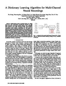
Fig. 2. The most correlated dictionary atoms (red) w.r.t the canonical HRF (blue) recovered by a) K-SVD, b) S1 , and c) Proposed algorithm.

4.2.2. Dictionary Learning In order to reduce the computation time for dictionary learning, the data matrix Y was down-sampled by a factor of 8 along the spatial direction. In all algorithms, the dictionary to be learned Dl ∈ Rm×40 was initialized with randomly selected data signals yi with columns normalized to have a unit l2 norm. The sparse coding step was done using correlation based thresholding [17, 18] with optimal sparsity level of k = 2 [17, 18] resulting in a sparse coefficient matrix X ∈ R40×N with Y = Dl X. In order to capture the remaining drift in the signals, the first element of the dictionary was set as DC and was never changed during the dictionary update stage. All algorithms were iterated 30 times with the S1 and proposed algorithms’ sparse coefficient and dictionary update steps 2 b) and 2 c) were iterated an additional 2 times per iteration. The hyper-parameters α1 = 0.2 and α2 = 0.22 were chosen for S1 and the proposed algorithm, with the proposed algorithm using the same value of α1 as used by S1 . We selected the most correlated dictionary atoms with respect to the canonical HRF from the recovered dictionaries and have presented them in Fig. 2. It can be seen that the proposed algorithm’s recovered atom is much smoother as compare to the atoms recovered by K-SVD and S1 . The sparse vectors x corresponding to the most correlated atoms were used to recover the activation maps with their z-thresholded maps presented in Fig. 3 where the neural activations in auditory cortex are identified correctly by all three algorithms, with the proposed method’s activations having higher specificity as compared to K-SVD. 5. CONCLUSION Data sets arising for example from spatio-temporal measurements as in fMRI studies can be structurally smooth. In this case the data set reshaped as a spatio-temporal matrix is struc-

1 0.9

(a)

0.8 0.7 0.6

(b)

0.5 0.4 0.3 0.2

(c) 0.1 0

Fig. 3. Z-statistics activation map for auditory stimulus of single subject at a random field correction p < 0.001 recovered by a) K-SVD, b) S1 , and c) Proposed algorithm

tured in the column domain and classical dictionary learning algorithms ignoring this structure in the data matrix will result in lower performance. Taking a regularized rank-one matrix approximation approach via penalization in the dictionary update stage a dictionary learning method adapted for data matrices whose column domain is structurally smooth was proposed in this paper. The obtained algorithm for the dictionary update stage can be seen as a variant of the power method or alternating least square method for computing the SVD in which smoothness via penalization is introduced. 6. REFERENCES [1] R. Baraniuk, V. Cevher, and M. Wakin, “Lowdimensional models for dimensionality reduction and signal recovery: A geometric perspective,” IEEE Proceedings, vol. 98, pp. 959–971, 2010. [2] I. Tosic and P. Frossard, “Dictionary learning,” IEEE Signal Processing Magazine, vol. 28, pp. 27–38, 2011. [3] M. Aharon, Michael Elad, and alfred Bruckstein, “KSVD: Anlgorithm for desiging overcomplete dictionaries for sparse representation,” IEEE Transactions on Signal Processing, vol. 54, pp. 4311–4322, 2006. [4] A. K. Seghouane and M. Hanif, “A sequential dictionary learning algorithm with enforced sparsity,” IEEE International Conference on Acoustic Speech and signal Processing, ICASSP, pp. 3876–3880, 2015. [5] K. Engan, S. O. Aase, and J. Hakon-Husoy, “Method of optimal directions for frame design,” IEEE Int. Conference on Acoustics, Speech, and Signal Processing, pp. 2443–2446, 1999.

[6] M. Hanif and A. K. Seghouane, “Maximum likelihood orthogonal dictionary learning,” IEEE Workshop on Statistical Signal Processing (SSP), pp. 1–4, 2014. [7] S. Ubaru, A. K. Seghouane, and Y. Saad, “Improving the incoherence of a learned dictionary via rank shrinkage,” Neural Computation, pp. 263–285, 2017. [8] M. U. Khalid and A. K. Seghouane, “A single SVD sparse dictionary learning algorithm for fMRI data analysis,” In Proceedings of IEEE International Workshop on Statistical signal Processing, pp. 65–68, 2014. [9] M. U. Khalid and A. K. Seghouane, “Constrained maximum likelihood based efficient dictionary learning for fMRI analysis,” In Proceedings of IEEE International Symposium on Biomedical Imaging, pp. 45–48, 2014. [10] A. K. Seghouane and Y. Saad, “Prewhitening high dimensional fmri data sets without eigendecomposition,” Neural Computation, vol. 26, pp. 907–919, 2014. [11] G. H. Golub and C. f. Van Loan, Matrix Computations, Johns Hopkins, 1996. [12] A. K. Seghouane and M. Bekara, “A small sample model selection criterion based on the kullback symmetric divergence,” IEEE Transactions on Signal Processing, vol. 52, pp. 3314–3323, 2004. [13] A. K. Seghouane and S. I. Amari, “The aic criterion and symmetrizing the kullback-leibler divergence,” IEEE Transactions on Neural Networks, vol. 18, pp. 97–106, 2007. [14] A. K. Seghouane, “Asymptotic bootstrap corrections of AIC for linear regression models,” Signal Processing, vol. 90, pp. 217–224, 2010. [15] M. R. Osborne, B. Presnell, and B. A. Turlach, “A new approach to variable selection in least squares problems,” IMA Journal of Numerical Analysis, vol. 20, 2000. [16] J. Tropp and S. J. Wright, “Computational methods for sparse solution of linear inverse problems,” Proceedings of the IEEE, vol. 98, pp. 948–958, 2010. [17] A. K. Seghouane and A. Iqbal, “Basis expansion approaches for regularized sequential dictionary learning algorithms with enforced sparsity for fMRI data analysis,” IEEE Transactions on Medical Imaging, pp. 1–12, 2017. [18] A. K. Seghouane and A. Iqbal, “Sequential dictionary learning from correlated data: Application to fmri data analysis,” IEEE Transactions on Image Processing, pp. 3002–3015, 2017.