Apr 26, 2006 ... Songwon Seo ... This paper reviews and compares several common and less
common outlier labeling methods ... Songwon Seo, M.S..
A Review and Comparison of Methods for Detecting Outliers in Univariate Data Sets
by Songwon Seo BS, Kyunghee University, 2002
Submitted to the Graduate Faculty of Graduate School of Public Health in partial fulfillment of the requirements for the degree of Master of Science
University of Pittsburgh 2006
UNIVERSITY OF PITTSBURGH Graduate School of Public Health This thesis was presented by Songwon Seo
It was defended on April 26, 2006 and approved by:
Laura Cassidy, Ph D Assistant Professor Department of Biostatistics Graduate School of Public Health University of Pittsburgh Ravi K. Sharma, Ph D Assistant Professor Department of Behavioral and Community Health Sciences Graduate School of Public Health University of Pittsburgh Thesis Director: Gary M. Marsh, Ph D Professor Department of Biostatistics Graduate School of Public Health University of Pittsburgh
ii
Gary M. Marsh, Ph D
A Review and Comparison of Methods for Detecting Outliers in Univariate Data Sets Songwon Seo, M.S. University of Pittsburgh, 2006
Most real-world data sets contain outliers that have unusually large or small values when compared with others in the data set. Outliers may cause a negative effect on data analyses, such as ANOVA and regression, based on distribution assumptions, or may provide useful information about data when we look into an unusual response to a given study. Thus, outlier detection is an important part of data analysis in the above two cases. Several outlier labeling methods have been developed. Some methods are sensitive to extreme values, like the SD method, and others are resistant to extreme values, like Tukey’s method.
Although these
methods are quite powerful with large normal data, it may be problematic to apply them to nonnormal data or small sample sizes without knowledge of their characteristics in these circumstances. This is because each labeling method has different measures to detect outliers, and expected outlier percentages change differently according to the sample size or distribution type of the data. Many kinds of data regarding public health are often skewed, usually to the right, and lognormal distributions can often be applied to such skewed data, for instance, surgical procedure times, blood pressure, and assessment of toxic compounds in environmental analysis. This paper reviews and compares several common and less common outlier labeling methods and presents information that shows how the percent of outliers changes in each method according to the skewness and sample size of lognormal distributions through simulations and application to real data sets. These results may help establish guidelines for the choice of outlier detection methods in skewed data, which are often seen in the public health field.
iii
TABLE OF CONTENTS
1.0 INTRODUCTION ................................................................................................................ 1 1.1 BACKGROUND .......................................................................................................... 1 1.2 OUTLIER DETECTION METHOD ......................................................................... 3 2.0 STATEMENT OF PROBLEM ........................................................................................... 5 3.0 OUTLIER LABELING METHOD .................................................................................... 9 3.1 STANDARD DEVIATION (SD) METHOD ............................................................. 9 3.2 Z-SCORE .................................................................................................................... 10 3.3 THE MODIFIED Z-SCORE..................................................................................... 11 3.4 TUKEY’S METHOD (BOXPLOT) ......................................................................... 13 3.5 ADJUSTED BOXPLOT ............................................................................................ 14 3.6 MADE METHOD ....................................................................................................... 17 3.7 MEDIAN RULE ......................................................................................................... 17 4.0 SIMULATION STUDY AND RESULTS FOR THE FIVE SELECTED LABELING METHODS .................................................................................................................................. 19 5.0 APPLICATION .................................................................................................................. 32 6.0 RECOMMENDATIONS ................................................................................................... 36 7.0 DISCUSSION AND CONCLUSIONS.............................................................................. 38 APPENDIX A .............................................................................................................................. 40 THE EXPECTATION, STANDARD DEVIATION AND SKEWNESS OF A LOGNORMAL DISTRIBUTION……………………………………………………………….40 APPENDIX B .............................................................................................................................. 42 MAXIMUM Z SCORE………………………………………………………………….42 APPENDIX C .............................................................................................................................. 44 CLASSICAL AND MEDCOUPLE (MC) SKEWNESS………………………………..44
iv
APPENDIX D .............................................................................................................................. 47 BREAKDOWN POINT………………………………………………………………….47 APPENDIX E .............................................................................................................................. 48 PROGRAM CODE FOR OUTLIER LABELING METHODS………………………...48 BIBLIOGRAPHY ....................................................................................................................... 51
v
LIST OF TABLES
Table 1: Basic Statistic of a Simple Data Set ................................................................................. 2 Table 2: Basic Statistic After Changing 7 into 77 in the Simple Data Set ..................................... 2 Table 3: Computation and Masking Problem of the Z-Score ....................................................... 11 Table 4: Computation of Modified Z-Score and its Comparison with the Z-Score ..................... 12 Table 5: The Average Percentage of Left Outliers, Right Outliers and the Average Total Percent of Outliers for the Lognormal Distributions with the Same Mean and Different Variances (mean=0, variance=0.22, 0.42, 0.62, 0.82, 1.02) and the Standard Normal Distribution with Different Sample Sizes. ................................................................................................................ 27 Table 6: Interval, Left, Right, and Total Number of Outliers According to the Five Outlier Methods......................................................................................................................................... 34
vi
LIST OF FIGURES
Figure 1: Probability density function for a normal distribution according to the standard deviation.......................................................................................................................................... 5 Figure 2: Theoretical Change of Outliers’ Percentage According to the Skewness of the Lognormal Distributions in the SD Method and Tukey’s Method ................................................ 7 Figure 3: Density Plot and Dotplot of the Lognormal Distribution (sample size=50) with Mean=1 and SD=1, and its Logarithm, Y=log(x). ........................................................................................ 8 Figure 4: Boxplot for the Example Data Set................................................................................. 13 Figure 5: Boxplot and Dotplot. (Note: No outlier shown in the boxplot).................................... 14 Figure 6: Change of theIintervals of Two Different Boxplot Methods ........................................ 16 Figure 7: Stnadard Normal Distribution and Lognormal Distributions........................................ 20 Figure 8: Change in the Outlier Percentages According to the Skewness of the Data................. 22 Figure 9: Change in the Total Percentages of Outliers According to the Sample Size ................ 25 Figure 10: Histogram and Basic Statistics of Case 1-Case 4........................................................ 32 Figure 11: Flowchart of Outlier Labeling Methods...................................................................... 37 Figure 12: Change of the Two Types of Skewness Coefficients According to the Sample Size and Data Distribution.
(Note: This results came from the previous simulation. All the values
are in Table 5 ) .............................................................................................................................. 46
vii
1.0
INTRODUCTION
This chapter consists of two sections: the Background and Outlier Detection Method. In the Background, basic ideas of an outlier are discussed such as definitions, features, and reasons to detect outliers. In the Outlier Detection Method section, characteristics of the two kinds of outlier detection methods are described briefly: formal and informal tests.
1.1
BACKGROUND
Observed variables often contain outliers that have unusually large or small values when compared with others in a data set. Some data sets may come from homogeneous groups; others from heterogeneous groups that have different characteristics regarding a specific variable, such as height data not stratified by gender. Outliers can be caused by incorrect measurements, including data entry errors, or by coming from a different population than the rest of the data. If the measurement is correct, it represents a rare event.
Two aspects of an outlier can be
considered. The first aspect to note is that outliers cause a negative effect on data analysis. Osbome and Overbay (2004) briefly categorized the deleterious effects of outliers on statistical analyses: 1) Outliers generally serve to increase error variance and reduce the power of statistical tests. 2) If non-randomly distributed, they can decrease normality (and in multivariate analyses, violate assumptions of sphericity and multivariate normality), altering the odds of making both Type I and Type II errors. 3) They can seriously bias or influence estimates that may be of substantive interest.
The following example simply shows how one outlier can highly distort the mean, variance, and 95% confidence interval for the mean. Let’s suppose there is a simple data set composed of data points 1, 2, 3, 4, 5, 6, 7 and its basic statistics are as shown in Table 1. Now, 1
let’s replace data point 7 with 77. As shown in Table 2, the mean and variance of the data are much larger than that of the original data set due to one unusual data value, 77. The 95% confidence interval for the mean is also much broader because of the large variance. It may cause potential problems when data analysis that is sensitive to a mean or variance is conducted.
Table 1: Basic Statistic of a Simple Data Set
Mean
Median
Variance
95 % Confidence Interval for the mean
4
4
4.67
[2.00 to 6.00]
Table 2: Basic Statistic After Changing 7 into 77 in the Simple Data Set
Mean
Median
Variance
95 % Confidence Interval for the mean
14
4
774.67
[-11.74 to 39.74]
The second aspect of outliers is that they can provide useful information about data when we look into an unusual response to a given study. They could be the extreme values sitting apart from the majority of the data regardless of distribution assumptions. The following two cases are good examples of outlier analysis in terms of the second aspect of an outlier: 1) to identify medical practitioners who under- or over-utilize specific procedures or medical equipment, such as an x-ray instrument; 2) to identify Primary Care Physicians (PCPs) with inordinately high Member Dissatisfaction Rates (MDRs) (MDRs = the number of member complaints / PCP practice size) compared to other PCPs.23 In summary, there are two reasons for detecting outliers. The first reason is to find outliers which influence assumptions of a statistical test, for example, outliers violating the normal distribution assumption in an ANOVA test, and deal with them properly in order to improve statistical analysis. This could be considered as a preliminary step for data analysis. The second reason is to use the outliers themselves for the purpose of obtaining certain critical information about the data as was shown in the above examples.
2
1.2
OUTLIER DETECTION METHOD
There are two kinds of outlier detection methods: formal tests and informal tests. Formal and informal tests are usually called tests of discordancy and outlier labeling methods, respectively. Most formal tests need test statistics for hypothesis testing. They are usually based on assuming some well-behaving distribution, and test if the target extreme value is an outlier of the distribution, i.e., weather or not it deviates from the assumed distribution. Some tests are for a single outlier and others for multiple outliers. Selection of these tests mainly depends on numbers and type of target outliers, and type of data distribution.1 Many various tests according to the choice of distributions are discussed in Barnett and Lewis (1994) and Iglewicz and Hoaglin (1993). Iglewicz and Hoaglin (1993) reviewed and compared five selected formal tests which are applicable to the normal distribution, such as the Generalized ESD, Kurtosis statistics, Shapiro-Wilk, the Boxplot rule, and the Dixon test, through simulations. Even though formal tests are quite powerful under well-behaving statistical assumptions such as a distribution assumption, most distributions of real-world data may be unknown or may not follow specific distributions such as the normal, gamma, or exponential. Another limitation is that they are susceptible to masking or swamping problems. Acuna and Rodriguez (2004) define these problems as follows: Masking effect: It is said that one outlier masks a second outlier if the second outlier can be considered as an outlier only by itself, but not in the presence of the first outlier. Thus, after the deletion of the first outlier the second instance is emerged as an outlier. Swamping effect: It is said that one outlier swamps a second observation if the latter can be considered as an outlier only under the presence of the first one. In other words, after the deletion of the first outlier the second observation becomes a non-outlying observation.
Many studies regarding these problems have been conducted by Barnett and Lewis (1994), Iglewicz and Hoaglin (1993), Davies and Gather (1993), and Bendre and Kale (1987). On the other hand, most outlier labeling methods, informal tests, generate an interval or criterion for outlier detection instead of hypothesis testing, and any observations beyond the interval or criterion is considered as an outlier. Various location and scale parameters are mostly employed in each labeling method to define a reasonable interval or criterion for outlier detection. There are two reasons for using an outlier labeling method. One is to find possible outliers as a screening device before conducting a formal test. The other is to find the extreme values away 3
from the majority of the data regardless of the distribution. While the formal tests usually require test statistics based on the distribution assumptions and a hypothesis to determine if the target extreme value is a true outlier of the distribution, most outlier labeling methods present the interval using the location and scale parameters of the data. Although the labeling method is usually simple to use, some observations outside the interval may turn out to be falsely identified outliers after a formal test when the outliers are defined as only observations that deviate from the assuming distribution. However, if the purpose of the outlier detection is not a preliminary step to find the extreme values violating the distribution assumptions of the main statistical analyses such as the t-test, ANOVA, and regression, but mainly to find the extreme values away from the majority of the data regardless of the distribution, the outlier labeling methods may be applicable. In addition, for a large data set that is statistically problematic, e.g., when it is difficult to identify the distribution of the data or transform it into a proper distribution such as the normal distribution, labeling methods can be used to detect outliers. This paper focuses on outlier labeling methods. Chapter 2 presents the possible problems when labeling methods are applied to skewed data. In Chapter 3, seven outlier labeling methods are outlined. In Chapter 4, the average percentages of outliers in the standard normal and log normal distributions with the same mean and different variances is computed to compare the outlier percentage of the selected five outlier labeling methods according to the degree of the skewness and different sample sizes. In Chapter 5, the five selected methods are applied to real data sets.
4
2.0
STATEMENT OF PROBLEM
Outlier-labeling methods such as the Standard Deviation (SD) and the boxplot are commonly used and are easy to use. These methods are quite reasonable when the data distribution is symmetric and mound-shaped such as the normal distribution. Figure 1 shows that about 68%, 95%, and 99.7% of the data from a normal distribution are within 1, 2, and 3 standard deviations of the mean, respectively. If data follows a normal distribution, this helps to estimate the likelihood of having extreme values in the data3, so that the observation two or three standard deviations away from the mean may be considered as an outlier in the data.
Figure 1: Probability density function for a normal distribution according to the standard deviation.
The boxplot which was developed by Tukey (1977) is another very helpful method since it makes no distributional assumptions nor does it depend on a mean or standard deviation.19 The lower quartile (q1) is the 25th percentile, and the upper quartile (q3) is the 75th percentile of the data. The inter-quartile range (IQR) is defined as the interval between q1 and q3. 5
Tukey (1997) defined q1-(1.5*iqr) and q3+(1.5*iqr) as “inner fences”, q1-(3*iqr) and q3+(3*iqr) as “outer fences”, the observations between an inner fence and its nearby outer fence as “outside”, and anything beyond outer fences as “far out”.31
High (2000) renamed the
19
The “outside” and “far out”
“outside” potential outliers and the “far out” problematic outliers.
observations can also be called possible outliers and probable outliers, respectively. This method is quite effective, especially when working with large continuous data sets that are not highly skewed.19 Although Tukey’s method is quite effective when working with large data sets that are fairly normally distributed, many distributions of real-world data do not follow a normal distribution.
They are often highly skewed, usually to the right, and in such cases the
distributions are frequently closer to a lognormal distribution than a normal one.21
The
lognormal distribution can often be applied to such data in a variety of forms, for instance, personal income, blood pressure, and assessment of toxic compounds in environmental analysis. In order to illustrate how the theoretical percentage of outliers changes according to the skewness of the data in the SD method (Mean ± 2 SD, Mean ± 3 SD) and Tukey’s method, lognormal distributions with the same mean (0) but different standard deviations (0.2, 0.4, 0.6, 0.8, 1.0, 1.2) are used for the data sets with different degrees of skewness, and the standard normal distribution is used for the data set whose skewness is zero. The computation of the mean, standard deviation, and skewness in a lognormal distribution is in Appendix A. According to Figure 2, the two methods show a different pattern, e.g., the outlier percentage of Tukey’s method increases, unlike the SD method. It shows that the results of outlier detection may change depending on the outlier detection methods or the distribution of the data.
6
Outlier (%)
10 9 8 7 6 5 4 3 2 1 0
2 SD Method (Mean ± 2 SD) 3 SD Method (Mean ± 3 SD) Tukey's Method (1.5 IQR) Tukey's Method (3 IQR) 0
5 10 Skewness
15
Figure 2: Theoretical Change of Outliers’ Percentage According to the Skewness of the Lognormal Distributions in the SD Method and Tukey’s Method
When data are highly skewed or in other respects depart from a normal distribution, transformations to normality is a common step in order to identify outliers using a method which is quite effective in a normal distribution. Such a transformation could be useful when the identification of outliers is conducted as a preliminary step for data analysis and it helps to make possible the selection of appropriate statistical procedures for estimating and testing as well.21 However, if an outlier itself is a primary concern in a given study, as was shown in a previous example in the identification of medical practitioners who under- or over-utilize such medical equipment as x-ray instruments, a transformation of the data could affect our ability to identify outliers. For example, 50 random samples (x) are generated through statistical software R in order to show the effect of the transformation.
The random variable X has a lognormal
distribution (Mean=1, SD=1), and its logarithm, Y=log(x), has a normal distribution. If the observations which are beyond the mean by two standard deviations are considered outliers, the expected outliers before and after transformation are totally different. As shown in Figure 3, while three observations which have large values are considered as outliers in the original 50 random samples(x), after log transformation of these samples, two observations of small values appear to be outliers, and the former large valued observations are no longer considered to be outliers. The vertical lines in each graph represent cutoff values (Mean ± 2*SD). Lower and
7
upper cutoff values are (-1.862268, 9.865134) and (-0.5623396, 2.763236), respectively, in the lognormal data(x) and its logarithm(y). Although this approach is not be affected by extreme values because it does not depend on the extreme observations after transformation, after an artificial transformation of the data, however, the data may be reshaped so that true outliers are not detected or other observations
0
5
10
0.3 0.1
dnorm(y, 1, 1, )
0.20 0.00 0.10
dlnorm(x, 1, 1, )
may be falsely identified as outliers.21
-2
-1
0
x
0
5
1
2
3
1
2
3
y
10
-2
-1
0
x
y
Figure 3: Density Plot and Dotplot of the Lognormal Distribution (sample size=50) with Mean=1 and SD=1, and its Logarithm, Y=log(x).
Several methods to identify outliers have been developed. Some methods are sensitive to extreme values like the SD method, and others are resistant to extreme values like Tukey’s method. The objective of this paper is to review and compare several common and less common labeling methods for identifying outliers and to present information that shows how the average percentage of outliers changes in each method according to the degree of skewness and sample size of the data in order to help establish guidelines for the choice of outlier detection methods in skewed data when an outlier itself is a primary concern in a given study.
8
3.0
OUTLIER LABELING METHOD
This chapter reviews seven outlier labeling methods and gives examples of simple numerical computations for each test.
3.1
STANDARD DEVIATION (SD) METHOD
The simple classical approach to screen outliers is to use the SD (Standard Deviation) method. It is defined as 2 SD Method: x ± 2 SD 3 SD Method: x ± 3 SD, where the mean is the sample mean and SD is the sample standard deviation. The observations outside these intervals may be considered as outliers. According to the Chebyshev inequality, if a random variable X with mean μ and variance σ2 exists, then for any k > 0,
P[| X − μ | ≥ kσ ] ≤
1 k2
P[| X − μ | < kσ ] ≥ 1 -
1 , k2
k >0
the inequality [1-(1/k)2] enables us to determine what proportion of our data will be within k standard deviations of the mean3. For example, at least 75%, 89%, and 94% of the data are within 2, 3, and 4 standard deviations of the mean, respectively. These results may help us determine the likelihood of having extreme values in the data3. Although Chebychev's therom is true for any data from any distribution, it is limited in that it only gives the smallest proportion of observations within k standard deviations of the mean22. In the case of when the distribution of a 9
random variable is known, a more exact proportion of observations centering around the mean can be computed. For instance, if certain data follow a normal distribution, approximately 68%, 95%, and 99.7% of the data are within 1, 2, and 3 standard deviations of the mean, respectively; thus, the observations beyond two or three SD above and below the mean of the observations may be considered as outliers in the data. The example data set, X, for a simple example of this method is as follows: 3.2, 3.4, 3.7, 3.7, 3.8, 3.9, 4, 4, 4.1, 4.2, 4.7, 4.8, 14, 15. For the data set, x = 5.46, SD=3.86, and the intervals of the 2 SD and 3 SD methods are (-2.25, 13.18) and (-6.11, 17.04), respectively. Thus, 14 and 15 are beyond the interval of the 2 SD method and there are no outliers in the 3 SD method.
3.2
Z-SCORE
Another method that can be used to screen data for outliers is the Z-Score, using the mean and standard deviation. Zi =
xi − x , where Xi ~ N (µ, σ2), and sd is the standard deviation of data. sd
The basic idea of this rule is that if X follows a normal distribution, N (µ, σ2), then Z follows a standard normal distribution, N (0, 1), and Z-scores that exceed 3 in absolute value are generally considered as outliers. This method is simple and it is the same formula as the 3 SD method when the criterion of an outlier is an absolute value of a Z-score of at least 3. It presents a reasonable criterion for identification of the outlier when data follow the normal distribution. According to Shiffler (1988), a possible maximum Z-score is dependent on sample size, and it is computed as (n − 1) / n . The proof is given in Appendix B. Since no z-score exceeds 3 in a sample size less than or equal to 10, the z-score method is not very good for outlier labeling, particularly in small data sets21. Another limitation of this rule is that the standard deviation can be inflated by a few or even a single observation having an extreme value. Thus it can cause a masking problem, i.e., the less extreme outliers go undetected because of the most extreme outlier(s), and vice versa. When masking occurs, the outliers may be neighbors. Table 3 shows
10
a computation and masking problem of the Z-Score method using the previous example data set, X. Table 3: Computation and Masking Problem of the Z-Score
i
Case 1 ( x =5.46, sd=3.86)
Case 2 ( x =4.73, sd=2.82)
xi
Z-Score
xi
Z-Score
1
3.2
-0.59
3.2
-0.54
2
3.4
-0.54
3.4
-0.47
3
3.7
-0.46
3.7
-0.37
4
3.7
-0.46
3.7
-0.37
5
3.8
-0.43
3.8
-0.33
6
3.9
-0.41
3.9
-0.29
7
4
-0.38
4
-0.26
8
4
-0.38
4
-0.26
9
4.1
-0.35
4.1
-0.22
10
4.2
-0.33
4.2
-0.19
11
4.7
-0.20
4.7
-0.01
12
4.8
-0.17
4.8
0.02
13
14
2.21
14
3.29
14
15
2.47
-
-
For case 1, with all of the example data included, it appears that the values 14 and 15 are outliers, yet no observation exceeds the absolute value of 3. For case 2, with the most extreme value, 15, among example data excluded, 14 is considered an outlier. This is because multiple extreme values have artificially inflated standard deviations.
3.3
THE MODIFIED Z-SCORE
Two estimators used in the Z-Score, the sample mean and sample standard deviation, can be affected by a few extreme values or by even a single extreme value. To avoid this problem, the median and the median of the absolute deviation of the median (MAD) are employed in the 11
modified Z-Score instead of the mean and standard deviation of the sample, respectively (Iglewicz and Hoaglin, 1993). MAD = median{| xi − ~ x |} , where ~ x is the sample median. The modified Z-Score ( M i ) is computed as Mi =
0.6745( xi − ~ x) , where E( MAD )=0.675 σ for large normal data. MAD Iglewicz and Hoaglin (1993) suggested that observations are labeled outliers
when| M i |>3.5 through the simulation based on pseudo-normal observations for sample sizes of 10, 20, and 40.21 The M i score is effective for normal data in the same way as the Z-score.
Table 4: Computation of Modified Z-Score and its Comparison with the Z-Score
i
xi
Z-Score
modified Z-Score
1
3.2
-0.59
-1.80
2
3.4
-0.54
-1.35
3
3.7
-0.46
-0.67
4
3.7
-0.46
-0.67
5
3.8
-0.43
-0.45
6
3.9
-0.41
-0.22
7
4
-0.38
0
8
4
-0.38
0
9
4.1
-0.35
0.22
10
4.2
-0.33
0.45
11
4.7
-0.20
1.57
12
4.8
-0.17
1.80
13
14
2.21
22.48
14
15
2.47
24.73
Table 4 shows the computation of the modified Z-Score and its comparison with the ZScore of the previous example data set. While no observation is detected as an outlier in the ZScore, two extreme values, 14 and 15, are detected as outliers at the same time in the modified ZScore since this method is less susceptible to the extreme values. 12
3.4
TUKEY’S METHOD (BOXPLOT)
Tukey’s (1977) method, constructing a boxplot, is a well-known simple graphical tool to display information about continuous univariate data, such as the median, lower quartile, upper quartile, lower extreme, and upper extreme of a data set. It is less sensitive to extreme values of the data than the previous methods using the sample mean and standard variance because it uses quartiles which are resistant to extreme values. The rules of the method are as follows: 1. The IQR (Inter Quartile Range) is the distance between the lower (Q1) and upper (Q3) quartiles. 2. Inner fences are located at a distance 1.5 IQR below Q1 and above Q3 [Q1-1.5 IQR, Q3+1.5IQR]. 3. Outer fences are located at a distance 3 IQR below Q1 and above Q3 [Q1-3 IQR, Q3+3 IQR]. 4. A value between the inner and outer fences is a possible outlier. An extreme value beyond the outer fences is a probable outlier. There is no statistical basis for the reason that Tukey uses 1.5 and 3 regarding the IQR to make inner and outer fences. For the previous example data set, Q1=3.725, Q3=4.575, and IQR=0.85. Thus, the inner fence is [2.45, 5.85] and the outer fence is [1.18, 7.13]. Two extreme values, 14 and 15, are identified as probable outliers in this method. Figure 4 is a boxplot generated using the statistical
0
5
10
15
software STATA for the example data set.
Figure 4: Boxplot for the Example Data Set
13
While previous methods are limited to mound-shaped and reasonably symmetric data such as the normal distribution21, Tukey’s method is applicable to skewed or non mound-shaped data since it makes no distributional assumptions and it does not depend on a mean or standard deviation. However, Tukey’s method may not be appropriate for a small sample size21. For example, let’s suppose that a data set consists of data points 1450, 1470, 2290, 2930, 4180, 15800, and 29200. A simple distribution of the data using a Boxplot and Dotplot are shown in Figure 5. Although 15800 and 29200 may appear to be outliers in the dotplot, no observation is
30,000
shown as an outlier in the boxplot.
20,000
29200
10,000
15800
0
4180 2930 2290 1470 1450
Figure 5: Boxplot and Dotplot. (Note: No outlier shown in the boxplot)
3.5
ADJUSTED BOXPLOT
Although the boxplot proposed by Tukey (1977) may be applicable for both symmetric and skewed data, the more skewed the data, the more observations may be detected as outliers,32 as shown in Figure 2. This results from the fact that this method is based on robust measures such as lower and upper quartiles and the IQR without considering the skewness of the data. Vanderviere and Huber (2004) introduced an adjusted boxplot taking into account the medcouple (MC)32, a robust measure of skewness for a skewed distribution.
14
When Xn={ x1 , x 2 ,..., x n } is a data set independently sampled from a continuous univariate distribution and it is sorted such as x1 ≤ x 2 ≤ ... ≤ x n , the MC of the data is defined as MC ( x1 ,..., x n ) = med
( x j − med k ) − (med k − xi ) x j − xi
,where med k is the median of Xn, and i
and j have to satisfy xi ≤ med k ≤ x j , and xi ≠ x j . The interval of the adjusted boxplot is as follows (G. Bray et al. (2005)): [L, U] = [Q1-1.5 * exp (-3.5MC) * IQR, Q3+1.5 * exp (4MC) * IQR] if MC ≥ 0 = [Q1-1.5 * exp (-4MC) * IQR, Q3+1.5 * exp (3.5MC) * IQR] if MC ≤ 0, where L is the lower fence, and U is the upper fence of the interval. The observations which fall outside the interval are considered outliers. The value of the MC ranges between -1 and 1. If MC=0, the data is symmetric and the adjusted boxplot becomes Tukey’s box plot. If MC>0, the data has a right skewed distribution, whereas if MC0, the data has a right skewed distribution, whereas if MC