A review of different methodologies used for calculation of wind power capacity credit Lennart S¨oder
Mikael Amelin
School of Electrical Engineering Royal Institute of Technology Stockholm, Sweden Email:
[email protected]
School of Electrical Engineering Royal Institute of Technology Stockholm, Sweden Email:
[email protected]
5000 Total load during the week
4000 Available capacity MW
Abstract— The aim of this paper is to describe, review and compare some methods that are currently used for calculation of wind power capacity credit and for using the results for economic analysis. The methods to be studied are the conventional method based on equivalent firm capacity and the method denoted ”secured capacity” used in the German dena study. The economic analysis concerning the capacity cost will also be analyzed.
3000 2000 Deficit, in total 40 hours 1000 0
0
20
40
60
80
I. I NTRODUCTION
II. C APACITY C REDIT OF WIND POWER The capacity credit of wind power refers to the capability of wind power to increase the reliability of the power system. For defining the capacity credit one can use the same method as for other types of power plants [3], [4]. Figure 1 illustrates an example of weekly load. The available capacity is set to 3250 MW and the load is the real hourly load in the western part of Denmark during the week starting 2 January 2003. The available capacity is not the real one but has been chosen in order to illustrate the capacity credit of a certain amount of
Fig. 1.
120
140
160
Capacity deficit without wind power
wind power. In this situation, there would have been a capacity deficit during 40h of that week. If, now, wind power is introduced into this system, the available capacity is increased, c.f. Figure 2. The figure 5000 4000
MW
How to calculate the capacity credit of wind power is discussed in many countries. Since the power system load continuously has to be met with an equivalent amount of production, there has to be enough capacity with a certain reliability in all power systems. If one source has a lower capacity credit than other sources, then this ”lack of enough capacity credit” can be denoted ”capacity cost” [8]. No technology is 100 % reliable, so an evaluation of the capacity credit and capacity cost of wind power must be relative to the reliability of alternative resources. The capacity cost or value of a certain technology is not only depending on its reliability but also on the correlation of the availability with the load and the other sources in the system. One original paper where the Effective Load Carrying Capability of Generating Units was defined was published by L. L. GARVER, in 1966 [3]. This basic method for calculation of the capacity credit is also relevant for wind power and has been applied by several authors. Here this method will be reviewed together with the alternative approach used in the German dena study. From the value of the capacity credit the capacity cost can be estimated and here a basic description together will be described, and the approach used in [8], [9], [10] will be commented.
100 h
Available capacity
3000 2000 Deficit, in total 27 hours 1000 Wind power production 0
0
20
40
60
80
100
120
140
160
h
Fig. 2.
Capacity deficit with wind power
includes the real wind power production during the same week illustrated in Figure 1. During this week, mean wind power production was 392 MW. On 31 December 2002, total installed wind power capacity was 1994 MW. during 2002, the mean wind power production in this area was PW = 396 MW (i.e. the selected week is representative regarding total wind energy). This amount of wind power resulted in a decrease in the number of hours with with capacity deficit, falling from 40h to 27h. This meas that the reliability of the power system has increased as a result of the installed wind power. If the reliability was acceptable before the installation of wind power, wind power production will enable the power system to meet a higher demand at the same reliability level. Figure 3 shows that if the load increases by 300 MW during each hour (compared with the load shown in Figure 1, the
5000
MW
4000
given probability distribution of the total available generation capacity, the secured capacity is defined so that
Available capacity
3000
P (Gtot ≥ Gsec ) = psec
2000 Deficit, in total 40 hours
where
1000 Wind power production 0
0
20
40
60
80
100
120
140
(1)
160
h
Fig. 3. Capacity deficit with wind power and load + 300 MW compared with situation illustrated in Figure 1
number of hours with a capacity deficit increases to 40. This means that the capacity credit measured as the equivalent load-carrying capability of 1994 MW is CW = 300 MW, corresponding to 15 % of installed capacity. This is slightly lower than results from other studies, which indicate capacity credits in the range of 18-24 % of installed capacity [5], [6]. There remains the question of how wind power can have a capacity when there are situations with no wind? It has to be kept in mind that for any power source there is a risk that it is not available during peak loads. The method used here to define capacity credit is exactly the same as the method that is used to define the capacity credit for other sources [3]. The example above shows that the number of hours with capacity deficit decreases, but not to zero, when the amount of wind power increase. During hour 60, for instance, there is no wind, and i does not matter whether the amount of wind power increases during this hour, since there is no wind. But the figures also show that during peak hours there is sometimes wind, which means that wind power can decrease the risk of a capacity deficit. In the figures, one week is used for illustrative purposes, but the data of a longer period, probably over several years, have to be used to be able to draw general conclusions. Example 2.1: Compare the capacity credit of the wind power in figures 2-3 with the capacity credit of a thermal power station with the same yearly energy production with 4 weeks of maintenance and a capacity availability of 92 %. Solution to example 2.1: The mean weakly wind power production for 2002, illustrated in figure 2, was PW = 392 MW, corresponding to a yearly production of 3469 GWh. Assuming a thermal power station with 4 weeks of maintenance and a capacity availability of 92 %, the installed capacity has to be PT = 466 MW in order to give the same yearly energy production. The capacity credit for this thermal power plant is around CT = 429 MW (92% of 466 MW). This means, for this example, that the capacity credit of wind power production, CW = 300 MW corresponds to approximately 70 % of the capacity credit for a thermal power plant with the same yearly energy production. III. S ECURED C APACITY OF WIND POWER IN THE DENA STUDY
The notion secured capacity is introduced in the German dena study [2] as a measurement of how much a certain power plant can increase the reliability of supply in a system. For a
Gtot = total available generation capacity, Gsec = secured capacity, psec = level of supply reliability. The interpretation of the secured capacity and the level of supply reliability is that if the load is equal to the secured capacity then the probability that the available units can cover the load equals psec . In [2], psec is varied between 97 % and 98 %. It must be noted that psec does not correspond to the traditional definition of supply reliability (i.e., the LOLP), since different load levels are not considered. To calculate the secured capacity of a generation system, the probability distribution of the total generation capacity must be known. If Gg , g = 1, , K, represent the available capacity in unit g, then the total available generation capacity is Gtot =
K X
Gg
(2)
g=1
The probability distribution of Gtot can be calculated using recursive convolution if Gg are independent random variables. For computational reasons it is preferable to assume that the probability distribution of each Gg is discrete. This is true for a thermal power plant (for which either the installed capacity is available or there is no capacity at all available), but requires a slight approximation for wind power plants. Assume that the probability distribution of Gg has ng states, Denote the probability of the i:th state by pg,i , and the available generation capacity of the unit by Gg,i Let fg (x) denote the frequency function after adding the g:th unit to the total generation capacity; fg (x) is then calculated according to the convolution formula ng X fg (x) = pg,i fg−1 (x − Gg,i (3) i=1
From 3, the secured capacity including K units is determined by finding the maximal value which fulfils the condition 1, i.e., Gsec subject to
= maximize t X fK (t) ≥ Psec
(4) (5)
t≥x
The secured capacity of a specific power plant is calculated by comparing the total secured capacity with and without that power plant. Example 3.1: The dena study [2] describes a system with three thermal units as in table I. What is the secured capacity of the third unit for a level of supply reliability equal to 97 % Solution to example 3.1: Calculate the probability distribution of the total available generation capacity with and without the third unit using the convolution formula 3. The results are shown in table II. We can see that the with only two units, the
Unit 1 2 3
Installed capacity [MW] 300 200 90 G ENERATING
Availability [%] 97 98 95
1 0.8 0.6
TABLE I U NITS IN E XAMPLE 3.1
0.4 0.2 0
x [MW]
0 90 200 290 300 390 500 590
Without third unit Cumulative Probability P probability f (t) f2 (x)[%] t≥x 2 [%] 0.06 100 0 99.94 2.94 99.94 0 97.00 1.94 97.00 0 95.06 95.06 95.06 0 0
With the third unit Cumulative Probability P probability, f (t) f3 (x) [%] t≥x 3 [%] 0.03 100 0.06 100.00 0.15 99.94 2.79 99.79 0.10 97.00 1.84 96.90 4.75 95.06 90.31 90.31
TABLE II T OTAL AVAILABLE GENERATION CAPACITY IN E XAMPLE 3.1
secured capacity is 300 MW, because the maximal capacity which is exceeded at least 97 % of the time is 300 MW. Including the third unit does not change the secured capacity of the system, because the maximal capacity which is exceeded at least 97 % of the time is still 300 MW. Hence, the secured capacity of the third unit is 300 300 = 0 MW. A. EQUIVALENT FIRM POWER The equivalent firm power a generating unit [3] is here used for comparison and defined as the capacity of a 100 % available power plant which has the same ability to decrease the LOLP of the system as the studied generating unit [3]. Consider a system with K generating units, where the total generation capacity is given by the random variable as in 3. Now, if an additional unit is added to this system, the risk of power deficit is given by LOLPK+1 = P (Gtot,K + GK+1 < D)
0
500
1000
Fig. 4.
1500
2000
2500
3000
Duration curve of load in example 3.2
Example 3.3: Assume the same system as in example 3.2. Calculate the secure capacity (97 % and 99 % security level) and the capacity credit for an extra 300 MW unit (97 % availability). Solution to example 3.3. The secure capacity in this extra unit is 200 MW (for both 97 % and 99 % security level). The LOLP becomes 0.15 % and the capacity credit equivalent firm capacity is 288 MW, i.e., slightly lower than 97 % of 300 MW. Example 3.4: Assume the same system as in example 3.2. Calculate the secure capacity (97 % and 99 % security level) and the capacity credit for an extra 200 MW unit (98 % availability). Solution to example 3.4. The secure capacity in this extra unit is 200 MW (for both 97 % and 99 % security level), i.e., the same as for the 300 MW unit in example 3.3. The LOLP becomes 0.43 % and the capacity credit equivalent firm capacity is 196 MW, i.e., 98 % of 200 MW. The conclusion from examples 3.3 and 3.4 is that the method of secure capacity gives rather strange results (same secure capacity in a 200 and 300 MW unit), while the equivalent firm capacity gives more realistic results. Example 3.5: Assume the same system as in example 3.2. Calculate the secure capacity (97 % and 99 % security level) and the capacity credit for an extra 500 MW wind power installation with a duration curve as in figure 5. The expected value of the wind power is 150.2 MW.
(6) 1
where is the random variable representing the available generation capacity of the additional unit. The equivalent firm power of the additional is then the value of the scalar x such that the total available capacity of K units plus a 100 % reliable supply source with the capacity x results in the same LOLP as for K + 1 units, i.e., P (Gtot,K + x < D) = P (Gtot,K + GK+1 < D)
(7)
Example 3.2: Assume a power system with 5 thermal power 300 MW units (97 % availability) and 5 thermal power 200 MW units (98 % availability). Calculate the secure capacity in this system at a security level of 97 % and 99 % and the LOLP with a load as shown in figure 4. Solution to example 3.2. The secure capacity in this system is 2200 MW (97 % security level) and 2000 MW (99 % security level) respectively. The LOLP becomes 1.30 %.
0.8 0.6 0.4 0.2 0
0
50
100
Fig. 5.
150
200
250
300
350
400
450
500
Duration curve of wind power in example 3.5
Solution to example 3.5. The secure capacity for the system including 500 MW wind power is 2216 MW (97 % security level) and 2052 MW (99 % security level) respectively. This means that the additional value of 500 MW wind power is 16 MW (97 % security level) and 52 MW (99 % security level) respectively. The LOLP becomes 0.75 % and the capacity credit equivalent firm capacity is 124 MW, which is lower
than the expected value of the wind power production. The conclusion from examples 3.5 is that the method of secure capacity gives higher secure capacity of wind power when the security level increased from 97 % to 99 %. The secure capacity of wind power is significantly lower than the capacity credit calculated as equivalent firm capacity. In [1] the method of how to calculate wind power capacity credit in the Nordic region is described. This corresponds to a simplified version of the method applied in the dena study. IV. O N CAPACITY COST FOR WIND POWER In example 2.1 it was shown that there were two possibilities to generate a certain amount of electric energy per year: wind power or thermal power. The capacity credit for the wind power alternative was in this case 30 % lower than the capacity credit for the thermal alternative. The capacity cost for wind power then can be seen as the cost of compensation for a comparatively lower capacity credit. The question is now if this can be considered as a problem, and what the costs are to solve this problem, if there is one. First concerning the size of the possible problem. A capacity credit only has a value if it sometimes is needed. If there is a large overcapacity installed in a certain system, then the value for the capacity credit will be very low, since there will always be a surplus of capacity in the system. In example 2.1 the difference in capacity credit corresponded to 429-300=129 MW. If there is a large over capacity in the system, then the value of this extra 129 MW in the thermal alternative has a very low value. But now assume that there are situations with low margins, which means that capacity is really important. In example 2.1 this means that since wind power has a capacity credit which is 129 MW lower than for thermal power, then the wind power alternative will result in slightly lower system reliability (a larger LOLP) than the thermal power alternative. The question is then the cost for this. First one then have to define the type of the problem and the cheapest way to solve it. The problem with a too high LOLP is that the risk of capacity (= expected number of minutes/hours per year when some load have to be disconnected because of capacity deficit), is unacceptably high. It must then be noted that this only occurs some minutes/hours per year, which means that one possible solution is to use gas turbines in order to compensate for the low capacity credit. It is not economic to invest in base power with much higher capacity costs, as e.g. coal power or nuclear power, to produce power that is only needed during some minutes/hours per year. Example 4.1: Calculate the capacity cost for wind power when the capacity credit is zero MW, and the compensation is performed with gas turbines with a cost of 33 Euro/kW,year (= investment cost). This is a common cost used in Sweden. Assume that the alternatives are 600 MW thermal base load plant (capacity credit around 0.95·600=570 MW), yearly production 7500h·600MW = 4.5 TWh/year) and 1400 MW of wind power (same yearly energy production, 2500h·1800 MW= 4.5 TWh/year).
Solution to example 4.1: In this example we have to add 570 MW of gas turbines in order to get the same capacity credit for the two options. The cost for this is 570 000 kW · 33 Euro/kW,year = 18.81 Meuro/year. This corresponds to 18.81/4,5 = 4.18 Euro/MWh. Example 4.2: Calculate the same as in example 4.1 but now with the assumption that the capacity credit is 15 % of installed capacity as in figure 2. Solution to example 4.2: A capacity credit of 15 % corresponds to 0.15·1800 MW = 270 MW. This means that, in order to get the same capacity credit as the conventional power plant, only 570-270=300 MW of gas turbines have to be built, corresponding to 2.2 Euro/MWh. In general it can be concluded that the capacity cost is a comparatively low cost even if the capacity credit is low. It must though be noted that the cost of gas turbines might be higher which may increase the capacity cost. But one must also note that the capacity cost is only larger than zero if there really is a need of the capacity! It is also important to note that if there are other, cheaper solutions than gas turbines, e.g., load reduction in extreme cases, then this will be used, which will also reduce the capacity cost. A. The capacity cost of wind power reported in [8], [9], [10] In [8] it is stated that The ILEX [9] and the GreenNet [10] studies assess the capacity costs of wind power. With a share of wind power of 20 % of the consumption the ILEX study assess the capacity costs in United Kingdom to 6.7 Euro/MWh of wind power. The GreenNet study assess the capacity cost of wind power in several EU countries to 3-4 Euro/MWh of wind power at shares of approximately 20 % of consumption. The explanation for these comparatively high figures is that the capacity credit for wind power is not calculated with a correct method and/or compensation is not performed in the cheapest possible way. It is not realistic to get these high figures when the real problem of lack of capacity credit is studied, i.e., possibility to get capacity in situations with extreme loads and/or many outages in conventional units. These situations are managed with comparatively cheap capacity, i.e., gas turbines and/or flexible load. V. C ONCLUSIONS • •
• •
•
The secured capacity of an additional unit is sensitive to the required reliability level. The secured capacity of an additional unit is not necessarily depending on the availability of the additional unit. The secured capacity of the system is not a measurement of the risk of power deficit (i.e., the LOLP). The secured capacity of a specific power plant does not account for the capability of the power plant to mitigate power deficit during off-peak periods. The conventional method denoted Effective Load Carrying Capability of Generating Units gives a more realistic, understandable, stable and correct estimation of the capacity credit than the secured capacity.
• •
•
It is important to consider the need of a capacity credit when a capacity cost is to be estimated. It is important to consider the capacity credit of wind power when the capacity cost of wind power is to be estimated. It is important to consider the cheapest way to compensate for lack of capacity credit when the capacity cost of wind power is to be estimated. ACKNOWLEDGMENT
This paper is performed within the framework of IEA Annex XXV Design and operation of power systems with large amounts of wind power B IOGRAPHY Lennart S¨oder (M 91) was born in Solna, Sweden in 1956. He received his M.Sc. and Ph.D. degrees in Electrical Engineering from KTH, Stockholm, Sweden in 1982 and 1988 respectively. He is currently a professor in Electric Power Systems at KTH. He works with projects concerning deregulated electricity markets, distribution systems and integration of wind power, HVDC, power system reliability, protections systems, hydro power and micro grids. He has been involved in several national committees concerning risk of capacity deficit and handling of bottlenecks within the deregulated market. Mikael Amelin received his M.Sc. and Ph.D. degrees in Electrical Engineering from KTH, Stockholm, Sweden in 1997 and 2004 respectively. He is currently a research associate in Electric Power Systems at KTH. He works with projects concerning deregulated electricity markets, integration of wind power, Monte-Carlo techniques, power system reliability, and rural electrification. R EFERENCES [1] Wind Power in Nordel - system impact for the year 2008, Nodel, 16 January 2007, available from www.nordel.org. [2] Planning of the Grid Integration of Wind Energy in Germany Onshore and Offshore up to the Year 2020 (dena Grid study) Deutsche EnergieAgentur GmbH, available from http://www.dena.de/de/themen/themakraftwerke/projekte/projekt/netzstudie-i/ (in German), (March 2005) [3] Garver, L. L. Effective Load Carrying Capability of Generating Units, IEEE Transactions on Power apparatus and Systems, Vol. PAS-85, no 8, (1966) [4] Milligan, M. R. (2002) Modeling Utility-Scale Wind Power Plants, Part 2: Capacity Credit. 67pp.; NICH Report No. TP-500-29701. Available on http://www.nrel.gov/publications/ [5] Munsgaard J., Mogens R., Pedersen, Pederson J. R. Economic value of wind power. Report 1, J. øAmternes of Kommunernes Forskningsinstitut, AKF rapport, (in Danish)(1995) [6] van Wijk Ad, Wind Energy and Electricity Production, PhD thesis, ISBN: 90-9003863-9, the Netherlands (1990) [7] S¨oder L. , The Value of Wind Power, in Wind Power in Power Systems, John Wiley & Sons, Ltd, ISBN:0-470-85508-8 (2005) [8] Projected Costs of Generating Electricity 2005 Update, International Energy Agency, available from www.iea.org, appendix 9: Economic Impacts of Wind Power Integration into Electricity Grids, ISBN 92-6400826-8 (2005) [9] ILEX Energy Consulting & Goran Strbac, Manchester Center of Electrical Energy, Quantifying the System Costs of Additional Renewables in 2020, A report to the Department of Trade & Industry, (October 2002) No. 080, www.dti.gov.uk/energy/developep/080scar report v2 0.pdf.
[10] Hans Auer, Michael Stadler, Gustav Resch, Claus Huber, Thomas Schuster, Hans Taus, Lars Henrik Nielsen, John Tidwell and Derk Jan Swider (February 2004), Cost and Technical Constraints of RESE Grid Integration, a report in the GreenNet study, Vienna, Austria, www.greennet.at/downloads/WP2%/20Report%20GreenNet.pdf.