Jan 16, 2012 - Instituto de Astrofısica de Canarias, Vıa Láctea S/N, La Laguna 38200, ... Departamento de Astrofısica, Universidad de la Laguna, La Laguna ...
Draft version January 17, 2012 Preprint typeset using LATEX style emulateapj v. 5/2/11
A ROBUST DETERMINATION OF THE SIZE OF QUASAR ACCRETION DISKS USING GRAVITATIONAL MICROLENSING enez-Vicente J. Jim´
arXiv:1201.3187v1 [astro-ph.CO] 16 Jan 2012
Departamento de F´ısica Te´ orica y del Cosmos. Universidad de Granada, Campus de Fuentenueva, 18071, Granada, Spain Instituto Carlos I de F´ısica Te´ orica y Computacional. Universidad de Granada, 18071, Granada, Spain
E. Mediavilla Instituto de Astrof´ısica de Canarias, V´ıa L´ actea S/N, La Laguna 38200, Tenerife, Spain Departamento de Astrof´ısica, Universidad de la Laguna, La Laguna 38200, Tenerife, Spain
˜ oz J. A. Mun Departamento de Astronom´ıa y Astrof´ısica, Universidad de Valencia, 46100 Burjassot, Valencia, Spain
C. S. Kochanek Department of Astronomy, The Ohio State University, 140 West 18th Avenue, Columbus, OH 43210, USA Center for Cosmology and Astroparticle Physics, The Ohio State University, 191 West Woodruff Avenue, Columbus, OH 43210, USA Draft version January 17, 2012
ABSTRACT Using microlensing measurements from a sample of 27 image-pairs of 19 lensed quasars we determine a maximum likelihood estimate for the accretion disk size of an average quasar of rs = 4.0+2.4 −3.1 light days at rest frame hλi = 1736˚ A for microlenses with a mean mass of hM i = 0.3M⊙ . This value, in good agreement with previous results from smaller samples, is roughly a factor of 5 greater than the predictions of the standard thin disk model. The individual size estimates for the 19 quasars in our sample are also in excellent agreement with the results of the joint maximum likelihood analysis. Subject headings: accretion, accretion disks — gravitational lensing: micro — quasars: general 1. INTRODUCTION
The thin disk (Shakura & Sunyaev 1973) is the standard model to describe the inner regions of quasars. This model predicts typical sizes for the accretion disks of luminous quasars of ∼1015 cm (∼0.4 light days) in the (observer frame) optical bands. However, recent measurements based on quasar microlensing are challenging this prediction. Based on a combined optical and X-ray study of microlensing in 10 quadruply lensed quasars, Pooley et al. (2007) found that the source of optical light is larger than expected from basic thin accretion disk models by factors of 3 to 30. Studying microlensing variability observed for 11 gravitationally lensed quasars Morgan et al. (2010) also found that the microlensing estimates of the disk size are larger (by a factor ∼4) than would be expected from thin disk theory. Other monitoring based studies focused on individual objects like QSO2237+0305 (Kochanek 2004, Anguita et al. 2008, Eigenbrod et al. 2008, Mosquera et al. 2009, Agol et al. 2009, Poindexter & Kochanek 2010), PG1115+080 (Morgan et al. 2008), RXJ1131−1231 (Dai et al. 2010), HE1104−1805 (Poindexter et al. 2008) or HE0435−1223 (Blackburne et al. 2011b) generally support these conclussions. From single-epoch optical/IR and X-Ray measurements, Blackburne et al. (2011a) used the wavelength dependence of microlensing (chromaticity) to study the structure of accretion disks in 12 4-image lensed quasars, finding disk sizes larger than predicted by nearly an order of magnitude. More detailed studies of individual
objects based in microlensing chromaticity (Eigenbrod et al. 2008, Poindexter et al. 2008, Mosquera et al. 2011, Mediavilla et al. 2011a, Mu˜ noz et al. 2011) also found that the size estimated from microlensing is substantially larger than the values predicted by the thin disk theory (by factors of about 10 in HE0435−1223, 5 in SBS0909+532, and 4 in HE1104−1805). Upper limits on the sizes of MG0414+0534 and SDSSJ0924+0219 have also been set by Bate et al. (2008) and Floyd et al. (2009), respectively. Here, we will generalize these results by extending the study to the sample of 20 lensed quasars of Mediavilla et al. (2009, hereafter MED09). Our data consists of microlensing amplitude measurements for 29 image-pairs from 20 lensed quasars based on a comparison between the flux ratios in the continuum and an adjacent emission line. The emission line flux ratio provides an unmicrolensed baseline that also removes the effects of extinction (see e.g. Falco et al. 1999, Mu˜ noz et al. 2004) and lens models in the determination of the magnification anomalies. As noted in previous works (Kochanek 2004, Eigenbrod et al. 2008, Blackburne et al. 2011a), studies favouring the selection of objects with noticeable magnification anomalies (or epochs with high microlensing activity) may lead to a bias towards smaller quasar size determinations. The fact that one object does not show microlensing magnification anomalies may be due to the fact that it is either too big or that it lies in a region without significant magnification fluctuations. Thus, non-detection of microlensing also puts constraints
2 on the size of the sources and should be taken into account. The MED09 sample is also unaffected by this bias (indeed the histogram of estimated microlensing magnifications in this sample peaks at ∆m = 0). However, the data from MED09 do not include, for most imagepairs, enough measurements at different wavelengths to address chromaticity. For this reason we will start discussing the impact of chromaticity on the determination of microlensing based sizes (§2) to show that size estimates are dominated by microlensing amplitude and are relatively independent of chromaticity. In §3 we will use the microlensing data from MED09 to calculate a maximum likelihood estimate of the accretion disk size. The estimate will be for the typical size of the accretion disk of an average quasar rather than that of any particular source. We also make individual size estimates for the 19 objects using a complementary Bayesian approach, finding excellent agreement with the likelihood analysis. The main conclusions are presented in §4. 2. SIZE DETERMINATION FROM SINGLE WAVELENGTH MICROLENSING MEASUREMENTS
We will base our analysis on the microlensing measurements inferred by MED09 from optical spectroscopy available in the literature (29 quasar image pairs seen through 20 lens galaxies). The microlensing magnification between two images 1 and 2 is calculated as ∆m = (m2 − m1 )micro = (m2 − m1 )cont − (m2 − m1 )line , where (m2 − m1 )line is the flux ratio in an emission line and (m2 − m1 )cont is the flux ratio of the continuum adjacent to the emission line. With this method the microlensing magnification is isolated from extinction and from the mean lensing magnification, as these effects affect the line and the adjacent continuum equally. The consistency of this procedure has been confirmed with mid-IR data (MED09). The histogram of observed microlensing magnifications in MED09 showed that 93% of the quasar image pairs have microlensing |∆m| ≤ 0.8 mag. In this section, we are going to use this statistical constraint to estimate quasar accretion disk sizes from single wavelength microlensing measurements. We will apply a statistical approach similar to that used by Mediavilla et al. (2011a) to a representative lens system. Therefore, we take for the lens a standard SIS with values κ1 = γ1 = 0.45 and κ2 = γ2 = 0.55 for the convergence and shear at the positions of the two images. These values are typical of the lenses in the MED09 (cf. their Table 4). For the redshifts of lens and source we have taken the values zl = 0.57 and zs = 1.76, which are the average values for the sample. Using these parameters for the macro lens, we generate microlensing magnifications maps at the positions of images 1 and 2 using the inverse polygon mapping algorithm described in Mediavilla et al. (2006) and Mediavilla et al. (2011b). The calculated maps are 2000×2000 pixels in size, with a pixel size of 0.5 light days, or equivalently 1.295×1015 cm. In the image plane, the covered area is the source plane area increased by factors 1.5(1 − κ ± γ)−1 . For the fraction of projected mass density in stars, α, we use current estimates (Pooley et al. 2009, MED09, Mosquera et al. 2011) and consider only the cases with α = 0.05 and α = 0.1. We used microlenses of 1M ⊙.
In order to describe the structure of the source, we model the accretion disk with a Gaussian profile I(R) ∝ exp(−R2 /2rs2 ), where the characteristic size rs is a wavelength dependent parameter (related to the half-light radius as R1/2 = 1.18rs ). The wavelength dependence of the disk size is parametrized by a power law with exponent p such that rs (λ) ∝ λp . We smooth the magnification maps with Gaussians scaled to two wavelengths λB and λR representing characteristic blue and red wavelengths. We choose λR /λB = 2.3, the ratio between Lyα and Mg II, which is roughly the wavelength range covered by observations in the optical band. We calculate the probability of observing microlensing magnifications ∆m = µ2 − µ1 (where µ1 and µ2 are the magnifications at the positions of image 1 and 2 respectively) at wavelengths λB and λR , namely, ∆mB and ∆mR , for a grid in the size at λB , rs (λB ), and the exponent p. We use a logarithmic grid in rs such that log rsi = 0.3×i for i = 0 · · · 11 (rsi in light days) and a linear grid in p such that pj = 0.25×j for j = 0 · · · 13. We restrict ourselves to the case |∆mB | > |∆mR |, as we assume that the size of the source increases with wavelength, and therefore the largest magnifications are expected for the smallest (i.e. bluest) sources1 . obs The probability of observing ∆mobs B and ∆mR in a i j model with parameters rs and p is given by Z Z 1 2 obs prsi ,pj (∆mobs , ∆m ) ∝ d∆m d∆mR Nij e− 2 χ , B B R (1) where χ2 =
2 2 (∆mB − ∆mobs (∆mR − ∆mobs B ) R ) + 2 2 σ∆m σ∆m obs obs B
(2)
R
Here, Nij is the number of trials with ∆mB and ∆mR for the case with parameters rsi and pj , and σ∆mobs and B σ∆mobs are the uncertainties in the observed microlensing R magnifications, for which we have taken a typical value of σ∆mobs = σ∆mobs =0.05 mags. B R The calculations are performed for a grid of pairs ∆mB , ∆mR with ∆mB = 0.2×k for k = −4 · · · 4 and ∆mR = 0.2×m for m = 0 · · · k (so we always have |m| < |k| and |∆mB | > |∆mR |) for α = 0.05 and α = 0.1. This range of values for the strength of microlensing covers the vast majority of observed cases as shown in the histogram of observed microlensing strengths in the sample of MED09 (their Fig. 1). Thus, the probabiobs lity distribution prsi ,pj (∆mobs B , ∆mR ) is calculated for 14×12×29×2 = 9744 cases. For each one of those cases obs (i.e. for every quadruplet (p, rs , ∆mobs B , ∆mR )), the 8 probability is calculated using 10 trials. The results for the case α = 0.05 are shown in Figure 1 for ∆mB > 0. We have shown only the right side of the full figure, as the cases with ∆mB < 0 are very similar to those with the same value of |∆mB | so that the scenario is fairly symmetric with respect to ∆mB = 0. For the case α = 0.1 the results are very similar but the peaks in the probability distributions are displaced towards slightly higher values of rs . 1
Inversions are possible but rare (see Poindexter et al. 2008)
3
obs Fig. 1.— Grid of two dimensional probability distributions pr i ,pj (∆mobs B , ∆mR ) for the 15 cases with ∆mB > 0 and α = 0.05. Each s column corresponds to the distribution for a given value of ∆mB indicated at the top of the column. Each row corresponds to the distribution for a given value of ∆mR indicated at the right. For each distribution the abcissae represent p from 0.0 to 3.25 and the ordinates represent log rs from 0.0 to 3.3 (rs in light days). The contour levels are drawn at intervals of 0.25σ (the contour at nσ is drawn at exp(−n2 σ2 /2) from the peak of the distribution). The contour at 1σ is thicker than the rest.
With the exception of the cases in which ∆mB = ∆mR , the distributions show a clear covariance in the sense that larger sizes imply lower values of the exponent p. We also see that larger values of ∆mB favour smaller values for the source size rs . The most important result from this figure is that the probability distribution with respect to the size rs is dominated by the strength of microlensing (∆mB ) with very little dependence on the amount of chromaticity. Conversely, the value of the chromaticity (∆mB − ∆mR ) is the main factor in determining the exponent p. Indeed, the most probable values of rs (values within 1σ around the maximum of the distributions in Figure 1)
remain roughly constant along each column in Figure 1 as we move through the different rows. That means that even if we lack information on chromaticity, we can still obtain valuable information on the size of the sources from measurements of microlensing at a single wavelength. Another interesting and robust result from Figure 1 is that, with the exception of the case with no detected microlensing (∆mB = 0), the maximums of the distributions are all located in a fairly restricted range in rs . Therefore, microlensing magnifications in the range 0 < |∆mB | ≤ 0.8 will p provide sizes inpa rather restricted range between ∼1 M/M⊙ and ∼16 M/M⊙ light days irrespective of chromaticity, with larger magnifications
4 favouring smaller sizes. 3. DISCUSSION
Based on the results of the previous section, it is possible to constrain the size of the sources from measurements of the microlensing strength at a single wavelength, even if we have no information on the amount of chromaticity present. As noted above (see also Kochanek 2004, Eigenbrod et al. 2008, Blackburne et al. 2011a), each single microlensing measurement is affected by a degeneracy between the range of possible magnifications and source size effects. Statistics of large samples of lensed quasars (like MED09) can be used to minimize this uncertainty. In particular, we are going to use a maximum likelihood method to estimate an average size from the product of the individual likelihood functions for each image pair. This method includes the cases with little or no microlensing that by themselves would give rise only to lower limits on the size on an equal footing with those showing significant microlensing. The microlensing magnifications in this sample have been calculated using the continuum to line flux ratios of different lines for different objects. As size is related to wavelength, we should ideally use objects with magnifications obtained from lines at similar wavelengths. On the other hand, to have good statistics, we should also try to keep the sample as large as possible. With these restrictions in mind, we have chosen a compromise in which we used all objects with magnifications measured in the wavelength range between Lyα (1216˚ A) to Mg II (2798˚ A). With this choice, the average rest wavelength is in the relatively narrow range of hλi = 1736±373˚ A, while we still keep 27 image pairs from 19 lensed quasars. The dispersion introduced by the effect of wavelength in the size estimate will be taken into account later. We then use the measured microlensing magnifications in these 27 pairs as observed ∆mB (where B stands now for the average wavelength hλi = 1736˚ A). We computed magnification maps for each one of the images of the 27 pairs individually taking the κ and γ values from MED09 (except for SBS0909+532 for which we take the values in Mediavilla et al. 2011a). We again consider only α = 0.05 and α = 0.1. The calculated maps are 2000×2000 pixels in size, with a pixel size of 0.5 light-days. We have used the same logarithmic grid in rs from §2, as well as a linear grid rsi = 1.0 + 2.0×i light days for i = 0 · · · 24. Using the magnification maps, the probability of observing a in image pair j for a microlensing magnification ∆mobs j model with parameter rsi is given by: Z 1 2 (3) prsi (∆mobs )∝ Ni e− 2 χ d∆m j where χ2 =
2 (∆m − ∆mobs j ) . 2 σ∆mobs
(4)
j
We can calculate a likelihood function for rs as Y prsi (∆mobs L(rsi ) ∝ j ), j
where j runs over the 27 image-pairs considered.
(5)
Fig. 2.— Likelihood functions for the size of the accretion disk log rs for α = 0.05 (continuous line) and α = 0.1 (dashed line) in the full sample of quasars by MED09.
The results of this procedure for α = 0.05 and α = 0.1 are shown in Figure 2. The maximum likelihood occurs +0.4 for log rs = 2.0+0.4 −0.8 and log rs = 2.3−0.8 (rs in light days) for α = 0.05 and α = 0.1 respectively. Taking into ac1/2 count that rs ∝ hM i where hM i is the mean mass of the microlenses, our results for the mean size of the 1/2 accretion disk of quasars are rs = 7.4+3.6 −4.1 (hM i/M⊙ ) +5.0 1/2 light days for α = 0.05 and rs = 10−5.5 (hM i/M⊙ ) for α = 0.1. When scaled for a mean microlens mass of hM i = 0.3M⊙, representative of the stellar populations in galaxies, the sizes of the accretion disks become +2.6 rs = 4.0+2.0 −2.2 light days and rs = 5.5−3.1 light days for α = 0.05 and α = 0.1, respectively, at our average wavelength hλi=1736˚ A. The intrinsic dispersion in λ in between the sources implies an additional dispersion in rs of about 20%. When taking this effect into account in the +3.1 error bars, we finally have rs = 4.0+2.4 −3.1 and rs = 5.5−3.7 light days for α = 0.05 and α = 0.1, respectively. Using equation (3) and a Bayesian approach with a logarithmic prior on rs (see e.g. Mediavilla et al. 2011a), we also made individual estimates of rs for each one of the 19 quasars in our sample. For those objects for which there are several image pairs, the probability distributions for the different pairs were combined into a single probability function for that object. The resulting values for hM i = 0.3M⊙ and α = 0.05 are presented in Table 1 and in Figure 3. It is worth noting that the average value of these individual estimates (hrs i = 4.2 ± 4.4 light days) is very close to the one obtained with the joint likelihood analysis (although the use of a linear prior would increase the individual size estimates by 80%). Note that the average size shrinks noticeably (by ∼30%) if the pairs with |∆mB | < 0.1 are excluded from the sample. Thus we confirm that favouring the selection of quasars with noticeable microlensing introduces a clear bias towards smaller sizes (Kochanek 2004, Eigenbrod et al. 2008, Blackburne et al. 2011a). In Figure 3 we com-
5 TABLE 1 Sizes for individual objects at 1736 ˚ A Object HE0047−1756 HE0435−1223 HE0512-3329 SDSS0806+2006 SBS0909+532 SDSSJ0924+0219 FBQ0951+2635 QSO0957+561 SDSSJ1001+5027 SDSSJ1004+4112 QSO1017−207 HE1104−1805 PG1115+080 SDSSJ1206+432 SDSSJ1353+1138 HE1413+117 BJ1422+231 SBS1520+530 WFIJ0233−4723
rs (1736)˚ A
MBH (109 M⊙ )
4.0+8.5 −2.7 4.4+5.6 −2.4 2.6+3.2 −1.4 1.4+1.9 −0.8 1.8+1.9 −1.0 10.1−4.6 a 1.8+2.9 −1.2 3.5+7.3 −2.3 +10.5 4.6−3.2 2.2+2.2 −1.1 3.2+6.02 −2.12 1.0+0.9 −0.5 2.3+2.6 −1.2 1.2+1.4 −0.6 7.5−4.4 a 2.7+2.7 −1.3 20.017.3 −9.2 2.4+3.5 −1.5 3.6+5.3 −2.2
1.38 0.50 .... .... 1.95 0.11 0.89 2.01 .... 2.02 1.68 2.37 0.92 .... .... 0.26 4.79 0.88 ....
Line (CIV) (CIV)
(Hβ) (MgII) (MgII) (CIV) (CIV) (CIV) (CIV) (CIV)
(CIV) (CIV) (CIV)
Note. — Sizes in light days for individual objects at 1736 ˚ A obtained from microlensing magnifications of image pairs. Black hole masses are taken from the summary in Mosquera & Kochanek (2011). Emission line used for the mass estimate is indicated in fourth column. a These values have been calculated for ∆m B = 0 and are lower limits rather than true estimates
pare our estimates with previous results. Estimates from the present work are indicated with filled symbols, and estimates from previous works with open symbols. We have taken black-hole masses from Table 1 in Mosquera & Kochanek (2011), which they take from Peng et al. (2006), Greene et al. (2010) and Assef et al. (2011). The thin line corresponds to the theoretical prediction for the thin disk model at 1736 ˚ A (with L/LE = 1 and η = 0.1). The thick line corresponds to the empirical fit by Morgan et al. (2010) scaled to hλi=1736 ˚ A using p = 4/3 Our estimates are in good agreement with previous results (Blackburne et al. 2011a, Mediavilla et al 2011a, Mosquera et al. 2011, Mu˜ noz et al. 2011, Morgan et al. 2010, Floyd et al. 2009, Anguita et al. 2008, Poindexter et al. 2008, Eigenbrod et al. 2008, Bate et al. 2008, and Kochanek 2004) and show a discrepancy with respect to the predictions of the thin disk model of approximately a factor of 5. 4. CONCLUSIONS
We performed a statistical analysis to estimate the average size of the accretion disks of lensed quasars from the large sample (MED09) of microlensing magnification measurements. We find that most information on the size of the accretion disk is contained in the amplitude of the microlensing magnification and fairly independent of the amount of chromaticity. From a statistical analysis using measured microlensing magnification strengths from 27 image pairs from 19 lensed quasars in the sample of MED09 we measured the average size of the accretion disk of lensed quasars at a
˚ as a function of Fig. 3.— Size of the accretion disk at 1736 A the mass of the black hole (from Mosquera & Kochanek 2011) for hM i = 0.3M⊙ . Results from our joint analysis are the solid triangle and square for α=0.05 and α=0.1 respectively. Our estimates for individual objets are shown as filled diamonds (or upward arrows for lower limits). Open triangles are from Blackburne et al. (2011a) for objects with available black hole masses in Mosquera & Kochanek (2011). The asterisk is the estimate for SBS0909 from Mediavilla et al. (2011a). Estimates for HE1104 by Mu˜ noz et al. (2011) and Poindexter et al. (2008) are shown as an open square and an X respectively. The estimate for HE0435 by Mosquera et al. (2011) is shown as an open circle. Upper half circle, lower half circle and star show the estimates for QSO2337 by Anguita et al. (2008), Kochanek (2004) and Eigenbrod et al. (2008) respectively. The estimate for Q0957 by Hainline et al. (2012) is shown as a bow tie. Downward arrows indicate the upper limits for MG0414 by Bate et al. 2008 (right) and for SDSSJ0924 by Floyd et al. 2009 (left). Thin line is the prediction from the thin disk model (with L/LE = 1 and η=0.1). The thick solid line is the fit from Morgan et al. (2010) with their measurements shown as pluses. The dashed lines showing the limits due to the uncertainty in the y-intercept.
rest wavelength of hλi=1736˚ A. For a typical mean mass in the stellar population of the lens of hM i = 0.3M⊙ , and taking into account the intrinsic dispersion in λ, we find +3.1 rs = 4.0+2.4 −3.1 and rs = 5.5−3.7 light days for α = 0.05 and α = 0.1 respectively. These estimates are in agreement with other studies (Blackburne et al. 2011a, Mediavilla et al 2011a, Mosquera et al. 2011, Mu˜ noz et al. 2011, Morgan et al. 2010, Floyd et al. 2009, Anguita et al. 2008, Poindexter et al. 2008, Eigenbrod et al. 2008, Bate et al. 2008, and Kochanek 2004) and again find that disks are larger than predicted by the thin disk theory. We have also estimated the sizes of the 19 individual objects in the sample to find that they are in very good statistical agreement with the result from the maximum likelihood analysis. This research was supported by the Spanish Ministerio de Educaci´on y Ciencia with the grants C-CONSOLIDER AYA2007-67625-C02-02, AYA200767342-C03-01/03, AYA2010-21741-C03/02. J.J.V. is also supported by the Junta de Andaluc´ıa through the FQM-
6 108 project. J.A.M. is also supported by the Generalitat Valenciana with the grant PROMETEO/2009/64.
C.S.K. is supported by NSF grant AST-1009756.
REFERENCES Agol, E., Gogarten, S. M., Gorjian, V., & Kimball, A. 2009, ApJ, 697, 1010 Anguita, T., Schmidt, R. W., Turner, E. L. et al. 2008, A&A, 480, 327 Assef, R. J., Denney, K. D., Kochanek, C. S. et al. 2011, ApJ, 742:93 Bate, N. F., Floyd, D. J. E., Webster, R. L. & Wyithe, J. S. B. 2008, MNRAS, 391, 1955 Blackburne, J. A., Pooley, D, Rappaport, S. & Schechter, P. L. 2011, ApJ, 729, 34 Blackburne, J. A., Kochanek, C. S., Chen, B., Dai, X., Chartas, G. 2011, arXiv:1112.0027v1 Dai, X., Kochanek, C. S., Chartas, G. et al. 2010, ApJ, 709, 278 Eigenbrod, A., Courbin, F., Meylan, G. et al. 2008, A&A, 490, 933 Falco, E. E., Impey, C. D., Kochanek, C. S. et al. 1999, ApJ, 523, 617 Floyd, D. J. E., Bate, N. F., & Webster, R. L. 2009, MNRAS, 398, 233 Greene, J. E., Peng, C. Y., & Ludwig, R. R. 2010, ApJ, 709, 937 Hainline L. J., Morgan C. W., Beach J. N. et al. 2010, ApJ, 744, 104 Kochanek, C. S. 2004, ApJ, 605, 58 Mediavilla, E., Mu˜ noz, J. A., Lopez, P., et al. 2006, ApJ, 653, 942 Mediavilla, E., Mu˜ noz, J. A., Falco, E., et al. 2009, ApJ, 706, 1451 Mediavilla, E., Mu˜ noz, J. A., Kochanek, C. S., et al. 2011a, ApJ, 730, 16
Mediavilla, E., Mediavilla, T., Mu˜ noz, J. A. et al. 2011b, ApJ, 741, 42 Morgan, C. W., Kochanek, C. S., Dai, X., Morgan, N. D., & Falco, E. E. 2008, ApJ, 689, 755 Morgan, C. W., Kochanek, C. W., Morgan N. D. & Falco E. E. 2010, ApJ, 712, 1129 Mosquera, A. M., Mu˜ noz, J. A., & Mediavilla, E. 2009, ApJ, 691, 1292 Mosquera, A. M. & Kochanek C. S. 2011, ApJ, 738, 96 Mosquera, A. M., Mu˜ noz, J. A., Mediavilla, E., Kochanek, C. S. 2011, ApJ,728, 145 Mu˜ noz, J. A., Falco, E. E., Kochanek, C. S., McLeod, B. A., & Mediavilla, E. 2004, ApJ, 605, 614 Mu˜ noz, J. A., Mediavilla, E., Kochanek, C. S., Falco, E. E. & Mosquera, A. M. 2011, ApJ, 742, 67 Peng, C. Y., Impey, C. D., Rix, H. W. et al. 2006, ApJ, 649, 616 Poindexter, S., Morgan, N. & Kochanek, C. S. 2008, ApJ, 673, 34 Poindexter, S. & Kochanek, C. S. 2010, ApJ, 712, 668 Pooley, D., Blackburne, J. A., Rappaport, S., & Schechter, P. L. 2007, ApJ, 661, 19 Pooley, D., Rappaport, S., Blackburne, J. et al. 2009, ApJ, 697, 1892 Shakura, N. I. & Sunyaev, R. A. 1973, A&A, 24, 337