speedups of this magnitude and has been able to ben-. e t from over a thousand processors. ...... 15] Laurie Hulbert and Earl Zmijewski. Limiting communica-.
A Scalable Parallel Algorithm for Sparse Cholesky Factorization� Anshul Gupta Vipin Kumar Department of Computer Science, University of Minnesota, Minneapolis, MN 55455
Abstract In this paper, we describe a scalable parallel algorithm for sparse Cholesky factorization, analyze its performance and scalability, and present experimental results of its implementation on a 1024-processor nCUBE2 parallel computer. Through our analysis and experimental results, we demonstrate that our algorithm improves the state of the art in parallel direct solution of sparse linear systems by an order of magnitude|both in terms of speedups and the number of processors that can be utilized e�ectively for a given problem size. This algorithm incurs strictly less communication overhead and is more scalable than any known parallel formulation of sparse matrix factorization. We show that our algorithm is optimally scalable on hypercube and mesh architectures and that its asymptotic scalability is the same as that of dense matrix factorization for a wide class of sparse linear systems, including those arising in all two- and three- dimensional nite element problems.
1 Introduction This paper describes a parallel algorithm for sparse Cholesky factorization that is optimally scalable for a wide class of sparse linear systems of practical interest. This algorithm incurs strictly less communication overhead than any known parallel formulation of sparse matrix factorization, and hence, can utilize a higher number of processors e�ectively. It is well known that dense matrix factorization can be implemented e�ciently on distributed-memory parallel computers [7, 23, 18]. In this paper, we show that the parallel Cholesky factorization algorithm described here is as scalable as the best parallel formulation of dense matrix factorization on both mesh and hypercube architectures. We also show that our algorithm is equally scalable for sparse matrices arising from two- and three-dimensional nite element problems. The performance and scalability analysis of our algorithm is supported by experimental results on up to 1024 processors of the nCUBE2 parallel computer. � This work was supported by Army Research O�ce under contract # DA/DAAH04-93-G-0080 and by the University of Minnesota Army High Performance Computing Research Center under contract # DAAL03-89-C-0038. Access to the nCUBE2 at Sandia National Labs was provided via DeSRA consortium.
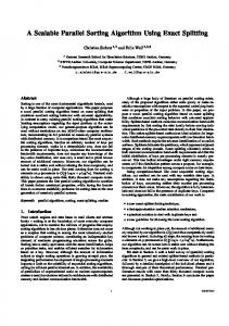
Global Mapping
Subtree-to-Subcube Mapping
Columnwise
Partitioning: 1-D
Partitioning
Mapping: Global
Mapping: Subtree-subcube
Communication overhead: Ω (Np log(p))
Communication overhead: Ω(Np)
Scalability: Ω ((p log(p)) 3 )
Scalability: Ω (p3 )
Partitioning: 2-D
Partitioning: 2-D
Partitioning in Both
A
C
Partitioning: 1-D
B
D
Mapping: Global
Mapping: Subtree-subcube
Communication overhead: Ω (Np 0.5 log(p))
Communication overhead: Θ (Np 0.5 )
Scalability: Ω (p 1.5 (log(p)) 3 ) Scalability: Θ (p1.5 )
Dimensions
Figure 1: An overview of the perfomance and scalability of parallel algorithms for factorization of sparse matrices resulting from two-dimensional N-node grid graphs. Box D represents our algorithm. We have been able to achieve speedups of up to 364 on 1024 processors and 230 on 512 processors over a highly e�cient sequential implementation for fairly small problems. A recent implementation of a variation of this scheme with improved load balancing reports 4{6 GFLOPS on moderate sized problems on a 256-processor Cray T3D [17]. To the best of our knowledge, this is the rst parallel implementation of sparse Cholesky factorization that has delivered speedups of this magnitude and has been able to bene t from over a thousand processors. Although we focus on Cholesky factorization of symmetric positive de nite matrices in this paper, the ideas presented here are can be adapted for sparse symmetric inde nite matrices [4] and nearly diagonally dominant matrices that are almost symmetric in structure [6, 13]. It is di�cult to derive analytical expressions for the number of arithmetic operations in factorization for general sparse matrices. This is because the computation and ll-in during the factorization of a sparse matrix is a function of the the number and position of nonzeros in the original matrix. In the context of the important class of sparse matrices that are adjacency matrices of graphs whose n-node subgraphs have O(pn)-node separators (this class includes sparse ma-
trices arising out of all two-dimensional nite di�erence and nite element problems), the contribution of this work can be summarized in Figure 1. A simple fan-out algorithm [9] with column-wise partitioning of an N � N matrix of this type on p processors results in an O(Np log N) total communication volume [11] (box A). The communication volume of the columnbased schemes represented in box A has been improved using smarter ways of mapping the matrix columns onto processors, such as, the subtree-to-subcube mapping [11] (box B). A number of column-based parallel factorization algorithms [21, 3, 25, 9, 8, 15, 14, 28] have a lower bound of O(Np) on the total communication volume. In [1], Ashcraft proposes a fan-both family of parallel Cholesky factorization algorithms that have a total communication volume of O(N pp log N). A few schemes with two-dimensional partitioning of the matrix have been proposed [22, 29, 27, 26], and the total communication volume in the best of these schemes [27, 26] is O(N pp logp) (box C). In summary, the simple parallel algorithm with O(Np logp) communication volume (box A) has been improved along two directions|one by improving the mapping of matrix columns onto processors (box B) and the other by splitting the matrix along both rows and columns (box C). In this paper, we describe a parallel implementation of sparse matrix factorization that combines the bene ts of improvements along both these lines. The total communication overhead of our algorithm is only O(N pp) for factoring an N � N matrix on p processors if it corresponds to a graph that satis es the separator criterion. Our algorithm reduces the communication overhead by a factor of at least O(logp) over the best algorithm implemented to date. It is also signi cantly simpler in concept as well as in implementation, which helps in keeping the constant factors associated with the overhead term low. Furthermore, as we show in Section 4.3, this reduction in communication overhead by a factor of O(logp) results in an improvement in the isoe�ciency metric of scalability [18, 12] by a factor of O((log p)3); i.e., the rate at which the problem size must increase with the number of processors to maintain a3constant ef ciency is lower by a factor of O((log p) ). This can make the di�erence between the feasibility and nonfeasibility of parallel sparse factorization on highly parallel (p � 256) computers.
2 The Multifrontal Algorithm for Sparse Matrix Factorization The parallel formulation presented in this paper is based on the multifrontal algorithm for sparse matrix factorization, which is described in detail in [20, 13, 5]. In this section, we brie y describe a simpli ed version of multifrontal sparse Cholesky factorization. Given a sparse matrix and the associated elimination tree, the multifrontal algorithm can be recur-
i 0 a+g i0
a
i1
b
d
i2
c
e
f
i0
i1
i2
+
i0
g
i2
h
j
i3
i
k
l
i0
i2
i3
i1
=
b
d
i 2 c+h
e
f+j
i3
i
0
k
l
i0
i1
i2
i3
Figure 4: The extend-add operation on two 3 � 3 triangular matrices. It is assumed that i0 < i1 < i2 < i3. sively formulated as shown in Figure 2. Consider the Cholesky factorization of an N � N sparse symmetric positive de nite matrix A into LL , where L is a lower triangular matrix. The algorithm performs a postorder traversal of the elimination tree associated with A. There is a frontal matrix F and an update matrix U associated with any node k. The row and column indices of F correspond to the indices of row and column k of L in increasing order. In the beginning, F is initialized to an (s + 1) � (s+1) matrix, where s+1 is the number of nonzeros in the lower triangular part of column k of A. The rst row and column of this initial F is simply the upper triangular part of row k and the lower triangular part of column k of A. The remainder of F is initialized to all zeros. After the algorithm has traversed all the subtrees rooted at a node k, it ends up with a dense (t + 1) � (t + 1) frontal matrix F , where t � N is the number of nonzeros in the strictly lower triangular part of column k in L. If k is a leaf in the elimination tree of A, then the nal F is the same as the initial F . Otherwise, the nal F for eliminating node k is obtained by merging the initial F with the update matrices obtained from all the subtrees rooted at k via an extend-add operation. The extend-add is an associative and commutative operation described in Figure 4. After F has been assembled, a single step of the standard dense Cholesky factorization is performed with node k as the pivot (lines 8{12, Figure 2). At the end of the elimination step, the column with index k is removed from F and forms the column k of L. The remaining t � t matrix is called the update matrix U and is passed on to the parent of k in the elimination tree. T
k
k
k
k
k
k
k
k
k
k
k
k
k
k
3 A Parallel Multifrontal Algorithm In this section we describe the parallel multifrontal algorithm for a p-processor hypercube. The algorithm also can be adapted for a mesh topology without any increase in the asymptotic communication overhead [13]. On other architectures as well, such as the CM-5, IBM SP-2 and Cray T3D, the asymptotic expression for the communication overhead remains the same. In this paper, we use the term supernode for a
% A is a sparse N � N symmetric positive de nite matrix to be factored. L is the lower triangular factor matrix such % that A = LL after factorization. A = (a ) and L = (l ), where 0 � i; j < N . Initially, all l = 0. 1. begin function 0 a Factor(k) a 1 a 2 ��� a s 1 BB a 1 0 0 � � � 0 CC 0 � � � 0 C; 2. F := B B@ a ..2 0.. .. . . . .. C . A . . . as 0 0 ��� 0 3. for all i such that Parent(i) = k in the elimination tree of A, do 4. begin 5. Factor(i); 6. F := Extend add(F , U ); 7. end % At this stage, F is a (t + 1) � (t + 1) matrix, where t is the number of nonzeros in the sub-diagonal part of column % k of L. U is a t � t matrix. Assume that an index i of F or U corresponds to the index q of A and L. 8. for i := 0 to t do p 9. L(q ; k) := F (i; 0)= F (0; 0); 10. for j := 1 to t do 11. for i := j to t do 12. U (i; j) := F (i; j) ? L(q ; k) � L(q ; k); 13. end function Factor. T
i;j
k;k
i;j
k;q
k;q
k;q
i;j
q ;k
k
q ;k
q ;k
k
k
i
k
k
k
k
i
k
k
i
k
k
i
j
Figure 2: An elimination-tree guided recursive formulation of the multifrontal sparse Cholesky algorithm. If r is the root of the postordered elimination tree of A, then a call to Factor(r) factors the matrix A. group of consecutive nodes in the elimination tree with one child. Henceforth, any reference to the height, depth, or levels of the tree will be with respect to the supernodal tree. For the sake of simplicity, we assume that the supernodal elimination tree is a binary tree up to the top log p supernodal levels. Any elimination tree can be converted to a binary supernodal tree suitable for parallel multifrontal elimination by a simple preprocessing step. In order to factorize the sparse matrix in parallel, portions of the elimination tree are assigned to processors using the standard subtree-to-subcube assignment strategy. This assignment is illustrated in Figure 3 for eight processors. With subtree-to-subcube assignment, all p processors in the system cooperate to factorize the frontal matrix associated with the topmost supernode of the elimination tree. The two subtrees of the root are assigned to subcubes of p=2 processors each. Each subtree is further partitioned recursively using the same strategy. Thus, the p subtrees at a depth of log p supernodal levels are each assigned to individual processors. A call to the function Factor given in Figure 2 with the root of a subtree as the argument generates the update matrix associated with that subtree. This update matrix contains all the information that needs to be communicated from the subtree in question to other columns of the matrix. After the independent factorization phase, pairs of processors (P2 and P2 +1 for 0 � j < p=2) perform a parallel extend-add on their update matrices, say Q j
j
and R, respectively. At the end of this parallel extendadd operation, P2 and P2 +1 roughly equally share Q + R. Here, and in the remainder of this paper, the sign \+" in the context of matrices denotes an extendadd operation. More precisely, all even columns of Q + R go to P2 and all odd columns of Q + R go to P2 +1. At the next level, subcubes of two processors each perform a parallel extend-add. Each subcube initially has one update matrix. The matrix resulting from the extend-add on these two update matrices is now merged and split among four processors. To e�ect this split, all even rows are moved to the subcube with the lower processor labels, and all odd rows are moved to the subcube with the higher processor labels. During this process, each processor needs to communicate only once with its counterpart in the other subcube. After this (second) parallel extend-add each of the processors has a block of the update matrix roughly one-fourth the size of the whole update matrix. Note that, both the rows and the columns of the update matrix are distributed among the processors in a cyclic fashion. Similarly, in subsequent parallel extend-add operations, the update matrices are alternatingly split along the columns and rows. This distribution is fairly straightforward to maintain. For example, during the rst two parallel extend-add operations, columns and rows of the update matrices are distributed depending on whether their least signi cant bit (LSB) is 0 or 1. Indices with LSB = 0 go j
j
j
j
0 1 2 3 4 5 6 7 8 9 10 11 12 13 14 15 16 17 18
X X X X X X X
X X X X X X X X X X X X X X X X X
Level 0
X X X X X X X X X X X X X X X X X
X X X
X X X X X
X X X X X X X X
X X X X X X X
X X X X X X X X X X X X X X X X X X X X X
0 1 2 3 4 5 6 7 8 9 10 11 12 13 14 15 16 17 18
P0,1,2,3,4,5,6,7
8
Level 1 X X X X X X
X
X X X
18
17
P0,1,2,3
7
6
Level 2
Level 3
2
P4,5,6,7
16
15
P0,1
5
P2,3
11
P4,5
14
P6,7
0
1
3
4
9
10
12
13
P0
P1
P2
P3
P4
P5
P6
P7
Figure 3: A symmetric sparse matrix and the associated elimination tree with subtree-to-subcube mapping onto 8 processors. The nonzeros in the original matrix are denoted by \�" and ll-ins by \�". to the lower subcube and those with LSB = 1 go to the higher subcube. Similarly, in the next two parallel extend-add operations, columns and rows of the update matrices are exchanged among the processors depending on the second LSB of their indices. Assume that the levels of the binary supernodal elimination tree are labeled starting with 0 at the top (Figure 3). In general, at level l of the supernodal elimination tree, 2log ? processors work on a single frontal or update matrix. These processors form a logical 2b(log ? ) 2c � 2d(log ? ) 2e mesh. The cyclic distribution rows and columns of these matrices among the processors helps maintain load-balance. The distribution also ensures that a parallel extend-add operation can be performed with each processor exchanging roughly half of its data only with its counterpart processor in the other subcube. Between two successive parallel extend-add operations, several steps of dense Cholesky elimination may be performed. The number of such successive elimination steps is equal to the number of nodes in the supernode being processed. The communication that takes place in this phase is the standard communication in pipelined grid-based dense Cholesky factorization [23, 18]. If the average size of the frontal matrices is t � t during the processing of supernode with m nodes on a q-processor subcube, then O(m) messages of size O(t=pq) are passed through the grid in a pipelined fashion. Figure 5 shows the communication for one step of dense Cholesky factorization of a hypothetical frontal matrix for q = 16. It is shown in [18] that although this communication does not take p
p
l =
l
p
l =
place between the nearest neighbors on a subcube, the paths of all communications on any subcube are con ict free with e-cube routing [18] and cut-through or worm-hole ow control. This is a direct consequence of the fact that a circular shift is con ict free on a hypercube with e-cube routing. Thus, a communication pipeline can be maintained among the processors of a subcube during the dense Cholesky factorization of frontal matrices. Further details of the parallel algorithm can be found in [13].
4 Communication Overhead and Scalability Analysis In this section, we analyze the communication overhead and the scalability of our algorithm on a hypercube for sparse matrices resulting from a nite di�erence operator on regular two{dimensional grids. Within constant factors, these expressions can be generalized to all sparse matrices that are adjacency matrices of graphs whose n-node subgraphs have an O(pn)-node separator because the properties of separators can be generalized from grids to all such graphs within the same order of magnitude bounds [19, 10]. In [13], we derive expressions for the communication overhead of this algorithm for three-dimensional grids and for the mesh architecture and show that the algorithm is optimally scalable in these cases as well. The parallel multifrontal algorithm described in Section 3 incurs two types of communication over-
0 0 1 2 3 2 8 9 12 3 10 11 14 15 4 0 1 4 5 0 5 2 3 6 7 2 3 6 8 9 12 13 8 9 12 7 10 11 14 15 10 11 14 15 8 0 1 4 5 0 1 4 5 0 9 2 3 6 7 2 3 6 7 2 10 8 9 12 13 8 9 12 13 8 11 10 11 14 15 10 11 14 15 10 0 1 2 3 4 5 6 7 8
Horizontal comunication 0 4 8
0
1
4
1 5 9
5
3 9 12 11 14 15 9 10 11
8
9
12
7
10
11
14
15
3
9
11
1
15
5
7
13
Vertical communication 0 4 8
0
2
8
1 5 9
10
0
(0,1,4,5), (2,3,6,7), (8,9,12,13),(10,11,14,15)
Vertical subcubes
6
0
Matrix indices
Horizontal subcubes
3 7 11
13
0
Processor numbers
3
0
0 3 6 10
2
3 6 10
(0,2,8,10), (1,3,9,11), (4,6,12,14),(5,7,13,15)
0
12
14
4
3 7 11
6
0
0
Figure 5: The two communication operations involved in a single elimination step (index of pivot = 0 here) of Cholesky factorization on a 12 � 12 frontal matrix distributed over 16 processors. head: one during parallel extend-add operations and the other during the steps of dense Cholesky factorization while processing the supernodes. Crucial to estimating the communication overhead is estimating the sizes of frontal and update matrices at any level of the supernodal tree. p p elimination Consider a N � N regular nite di�erence grid. We analyze the communication overhead for factorizing the N � N sparse matrix associated with this grid on p processors. In order to simplify the analysis, we assume a somewhat di�erent form of nesteddissection than the one used in the actual implementation. This method of analyzing the communication complexity of sparse Cholesky factorization has been used in [11]. Within very small constant factors, the analysis holds for the standard nested dissection [10] of grid graphs. We consider a cross-shaped separator p (described in [11]) consisting of 2 N ? 1 nodes that partitions thepN-node square p grid into four square subgrids of size ( N ? 1)=2 � ( N ? 1)=2. We call this the level-0 separator that partitions the original grid (or the level-0 grid) into four level-1 grids. The subgrids are further partitioned in the same way, and the process is applied recursively. The supernodal elimination tree corresponding to this ordering is such that each non-leaf supernode has four The p child supernodes. p topmost supernode has 2 N ? 1 (� 2 N) nodes, and the size of the supernodes at each subsequent supernodal level of the tree is half of the supernode size at the previous level. Clearly, the number of supernodes increases by a factor of four at each level, starting with one at the top (level 0). The nested dissection scheme described above has the following properties: (1) the size of level-l subgrids
p
p
is approximately N=2 � N=2 , (2) the number p of nodes in a level-l separator is approximately 2 N=2 , and hence, the length of a supernode at level p l of the supernodal elimination tree is approximately 2 N=2 . It has been proved in [11] that the number of nonzeros that an i � i subgrid can contribute to the nodes of its bordering separators is bounded by ki2 , where k = 341=12. Hence, a level-l subgrid can contribute at most kN=4 nonzeros to its bordering nodes. These nonzeros are in the form of the triangular update matrix that is passed along from the root of the subtree corresponding to the subgrid to its parent in the elimination tree. The dimensions of a matrix with a dense triangular part p containing kN=4 entries is roughly p 2kN=2 � 2kN=2 . Thus, the size of an update matrix passed on to level l ? 1 of the supernodal elimination tree p from level l is roughly upper-bounded by p 2kN=2 � 2kN=2 for l � 1. p The length p of a level-l supernode is 2 N=2 ; hence, a total of 2 N=2 elimination steps take place while the computation proceeds from the bottom of a level-l supernode to its top. A single elimination step on a frontal matrix of size (t+1)�(t+1) produces an update matrix of size t � t. Since the size of a frontal p matrix 2kN=2 � at the top of a level-l supernode is at most p 2kN=2 , the size of the frontal matrix at the bottom p of pthe samepsupernode p is upper-bounded by ( 2k ? 2) N=2 �( 2k ?2) N=2 . Hence, the average size of a frontal matrix at level l of p the supernodal p p elimination tree is upper-bounded by ( 2k ? 1) p p p N=2 � (p 2k ? 1) N=2 . Let 2k ? 1 = �. Then � N=2 � � N=2 is an upper bound on the average size of a frontal matrix at level l. l
l
l
l
l
l
l
l
l
l
l
l
l
l
l
l
l
l
l
l
4.1 Overhead in parallel extend-add Before the computation corresponding to level l ? 1 of the supernodal elimination tree starts, a parallel extend-add operation is performed triangular p on lower p 2kN=2 , � portions update matrices of size 2kN=2 each of which is distributed on a pp=2 � pp=2 logical mesh of processors. Thus, each processor holds roughly (kN=4 ) � (p=4 ) = kN=p elements of an update matrix. Assuming that each processor exchanges roughly half of its data with the corresponding processor of another subcube, t +t kN=(2p) time is spent in communication, where t is the message startup time and t is the per-word transfer time. Note that this time is independent of l. Since there are (logp)=2 levels at which parallel extend-add operations take place, the total communication time for these operations is O(N=p) log p on a hypercube. The total communication overhead due to the parallel extend-add operations is O(N log p) on a hypercube. l
l
l
l
l
l
s
w
s
w
4.2 Overhead in factorization steps
l
l
l
l
l
l
l
p
S
c
l
l
l
4.3 Scalability analysis The scalability of a parallel algorithm on a parallel architecture refers to the capacity of the algorithmarchitecture combination to e�ectively utilize an in-
c
P
o
P
S
P
o
P
o
S
S
o
We have shown earlier that the average size of a frontal matrix at level l ofpthe supernodal p elimination tree is bounded by � N=2 � � N=2 , where p ? 1. This matrix is distributed on a �p = 341=6 p=2 � pp=2 logical mesh of processors. As shown in Figure 5, there are two communication operations involved with each elimination step pof dense Cholesky. The average size of a message is (� N=2 ) � (pp=2 ) p = � N=p. It can be shown [23, 18] that in a pipelined implementation on a pq � pq mesh of processors, the communication time for s elimination steps with an average message size of m is O(ms). In our case, at level l of the supernodal elimination p tree, the number of steps of dense Cholesky is 2 N=2 . Thus pthe total communication time at level p p l is � N=p � 2 N=2 = O((N= p)(1=2 )). The total communication time for the elimination steps at top (log p)=2 levels of the supernodal elimination tree is log4 ?1 O((N=pp)� (1=2 )). This has an upper bound =0 p overof O(N= p). Hence, the total communication head due the elimination steps is O(N pp). The parallel multifrontal algorithm incurs an additional overhead of emptying the pipeline logp times (once before each parallel extend-add) and then re lling it. It can be easily shown that this overhead is is smaller in magnitude than the O(N pp) communication overhead of the dense Cholesky elimination steps [13]. l
creasing number of processors. In this section we use the isoe�ciency metric [18, 12] to characterize the scalability of our algorithm. Let W be the size of a problem in terms of the total number of basic operations required to solve a problem on a serial computer. The serial run time of a problem of size W is given by T = t W, where t is the time to perform a single basic computation step. If T is the parallel run time of the same problem on p processors, then we de ne an overhead function T as pT ? T . Both T and T are functions of W and p, and we often write them as T (W; p) and T (W; p), respectively. The e�ciency of a parallel system with p processors is given by E = T =(T + T (W; p)). If a parallel system is used to solve a problem instance of a xed size W, then the e�ciency decreases as p increases. For many parallel systems, for a xed p, if the problem size W is increased, then the e�ciency increases. For these parallel systems, the e�ciency can be maintained at a desired value (between 0 and 1) for increasing p, provided W is also increased. Given that E = 1=(1 + T (W; p)=(t W)), in order to maintain a xed e�ciency, W should be proportional to T (W; p). In other words, the following relation must be satis ed in order to maintain a xed e�ciency: W = te T (W; p); (1) o
c
o
o
c
where e = E=(1 ? E) is a constant depending on the e�ciency to be maintained. Equation (1) is the central relation that is used to determine the isoe�ciency function of a parallel algorithm-architecture combination. It is well known [10] that the total work involved in factoring pthe adjacency matrix of an N-node graph using nested dissecwith an O( N)-node separator tion ordering of nodes is O(N 1 5). We have shown in Section 4 that the overall communication overhead of our scheme is O(N pp). From Equation 1, a xed e�ciency if and only if N 1 5 / N pp, p canpbe maintained or N / p, or N 1 5 = W / p1 5. In other words, the problem size must be increased as O(p1 5) to maintain a constant e�ciency as p is increased. In comparison, a lower bound on the isoe�ciency function of Rothberg and Gupta's scheme [27] with a communication overhead of at least O(N pp log p) is O(p1 5(log p)3). The isoe�ciency3 function of any column-based scheme is at least O(p ) because the total communication overhead has a lower bound of O(Np). Thus, the scalability of our algorithm is superior to that of the other schemes. A lower bound on the isoe�ciency function for dense matrix factorization is O(p1 5) [18]. The factorization of a sparse matrix involves factoring a dense matrix and the amount of computation required to factor this dense matrix is of the same order as the amount of computation required 1to5 factor the entire sparse matrix [10, 11]. Hence, O(p ) is a lower bound :
:
:
:
:
:
:
:
Matrix:
p Time Speedup Efficiency Matrix:
p
GRID127x127; N = 16129; NNZ = 518.58 thousand; FLOP =36.682 million
1
4
8
16
32
64
128
256
58.86
15.07
8.878
5.155
2.971
1.783
1.171
.8546
1.00 100.0%
3.90 97.6%
6.63 82.8%
11.4 71.0%
19.8 61.9%
33.0 51.6%
50.3 39.3%
68.9 26.9%
GRID255x127; N = 32385; NNZ = 1140.6 thousand; FLOP =100.55 million
1
16
32
64
128
256
512
1024
Time Speedup
149.15 1.00
12.22 12.2
6.651 22.4
3.861 38.6
2.349 63.5
1.557 95.8
1.091 136.7
.8357 178.5
Efficiency
100.0%
76.3%
70.1%
60.4%
49.6%
37.4%
26.7%
17.4%
Figure 6: Experimental results for factoring sparse symmetric positive de nite matrices associated with a 9-point di�erence operator on rectangular grids. All times are in seconds. on the isoe�ciency function of sparse matrix factorization, and our algorithm achieves this bound.
5 Experimental Results We implemented the parallel multifrontal algorithm described in this paper on the nCUBE2 parallel computer and have gathered some preliminary speedup results for two classes of sparse matrices, which we summarize in Figures 6 and 8. The reader is referred to [13] for more detailed experimental results and their interpretations. We conducted one set of experiments on sparse matrices associated with a 9-point di�erence operator on rectangular grids (Figure 6). Matrix GRIDixj in the gure refers to the sparse matrix obtained form an i�j grid. The standard nested dissection ordering [10] was used for these matrices. The purpose of these experiments was to compare their results with the scalability analysis in Section 4.3. From our experiments on the 2-D grids, we selected a few points of equal e�ciency and plotted the W versus p curve, which is shown by the solid line in Figure 7 for E � 0:31. The problem size W is measured in terms of the total number of oating point operations required for factorization. The dotted and dashed curves indicate the problem sizes that will yield the same e�ciency for p 1=5 128, 256,1and 512 if the isoe�ciency function is O(p ) and O(p 5(log p)3), respectively. Figure 7 shows that our experimental isoe�ciency curve is considerable better than O(p1 5(log p)3 ), which is a lower bound on the isoe�ciency function of the previously best known (in terms of total communication volume) parallel algorithm [27] for sparse 1matrix factorization. However, it is worse than O(p 5), which is the asymptotic isoe�ciency function derived in Section 4.3.1 5There are two main reasons for this. First, the O(p ) isoe�ciency function does not take :
:
:
:
:
load imbalance into account. It has been shown in [21] that even if a grid graph is perfectly partitioned in terms of the number of nodes, the work load associated with each partition varies. Another reason is that the e�ciencies of the parallel implementation are computed with respect to a very e�cient serial implementation. In our implementation, the computation associated with the subtrees below level logp in the supernodal elimination tree is handled by the serial code. However, the computation above this level is handled by a separate code. In our preliminary implementation, this part of the code is less e�cient than the serial code (disregarding communication) due to additional bookkeeping, which has a potential for optimization. For example, the total time spent by all the processors participating in a parallel extend-add operation besides message passing is more than the time taken to perform extend-add on the same update matrices on a single processor. The same is true for the dense factorization steps too. However, despite these ine�ciencies, our implementation is more scalable than a hypothetical ideal implementation (with perfect load balance) of the currently best known parallel algorithm for sparse Cholesky factorization. In Figure 8 we summarize the results of factoring some matrices from the Harwell-Boeing collection of sparse matrices. The purpose of these experiments was to to demonstrate that our algorithm can deliver good speedups on hundreds of processors for practical problems. Spectral nested dissection (SND) [24] was used to order the matrices in Figure 8. From the experimental results in Figures 6 and 8, we can infer that our algorithm can deliver substantial speedups, even on moderate problem sizes. These speedups are computed with respect to a very e�cient serial implementation of the multifrontal algorithm. To lend credibility to our speedup gures, we compared the run times of our program on a single processor with the single processor run times
350 O(p 1.5 (log(p)) 3)
300
Experimental 250
O(p 1.5)
200 150
W
100
(in million 50 floating point ops) 0
50
100
150
200
250
300
350
400
450
500
550
p
Figure 7: Comparison of our experimental isoe�ciency curves with O(p1 5) curve (theoretical asymptotic isoe�ciency function of our algorithm due to communication overhead on a hypercube) and with O(p1 5(log p)3 ) curve (the lower bound on the isoe�ciency function of the best known parallel sparse factorization algorithm until now). The four data points on the curves correspond to the matrices GRID63x63, GRID103x95, GRID175x127, and GRID223x207. :
:
given for iPSC/2 in [25]. The nCUBE2 processors are about 2 to 3 times faster than iPSC/2 processors and our serial implementation, with respect to which the speedups are computed, is 4 to 5 times faster than the one in [25]. Our single processor run times are four times less than the single processor run times on iPSC/2 reported in [2]. We also found that for some matrices (e.g., that from a 127 � 127 9-point nite di�erence grid), our implementation on eight nCUBE2 processors (8.9 seconds) is faster than the 16-processor iPSC/860 implementation (9.7 seconds) reported in [29], although iPSC/860 has much higher computation speeds. The factorization algorithm as described in this paper requires a binary supernodal elimination trees that are fairly balanced. After obtaining the ordered matrix and the corresponding eliminationtree, we run the elimination tree through a very fast tree balancing algorithm, which is described in [13]. Figure 8 also gives the upper bound on e�ciency due to load imbalance for di�erent values of p for BCSSTK15, BCSSTK25, and BCSSTK29 matrices. It is evident from the load balance values given in Figure 8 that a combination of spectral nested dissection with our tree balancing algorithm results in very respectable load balances for up to 1024 processors. The number of nonzeros in the triangular factor (NNZ) and the number of oating point operations (FLOP) reported in Figure 8 are for the single processor case. As the number of processors is increased, the tree balancing algorithm is applied to more levels (logp) of the supernodal elimination tree, and consequently, the total NNZ and FLOP increase. Thus, an e�ciency of x% in Figure 8 indicates that there is a (100 ? x)% loss, which includes three fac-
tors: communication, load imbalance, and extra work. For example, the e�ciency for BCSSTK25 on 64 processors is 57%; i.e., there is a 43% overhead. However, only 5% overhead is due to communication and extra work. The remaining 38% overhead is due to load imbalance.
6 Concluding Remarks In this paper, we analytically and experimentally demonstrate that scalable parallel implementations of direct methods for solving large sparse systems are possible. In [28], Schreiber concludes that it is not yet clear whether sparse direct solvers can be made competitive at all for highly (p � 256) and massively (p � 4096) parallel computers. We hope that, through this paper, we have given an a�rmative answer to at least a part of the query. Our algorithm is a signi cant improvement over other parallel algorithms for sparse matrix factorization. This improvement has been realized by reducing the order of the communication overhead. An e�cient parallel sparse matrix factorization algorithm requires the following: (1) the matrix must be partitioned among the processors along both rows and columns because pure column-based partitioning schemes have much higher communication overhead [28, 27], (2) the distribution of rows and columns of the matrix among the processors must follow some sort of cyclic order to ensure proper load balance, and (3) communication must be localized among as few processors as possible at every stage of elimination by following a subtree-to-
Matrix:
p Time Speedup
1
2
4
8
16
32
64
128
256
103.73
52.63
26.66
14.88
8.29
4.98
3.20
2.156
1.530
1.00
Efficiency 100.0% Load balance
100%
1.97
3.89
6.97
12.5
20.8
32.4
48.1
67.8
98.5%
97.3%
87.1%
78.2%
65.1%
50.7%
37.6%
26.5%
99%
98%
91%
91%
87%
87%
84%
84%
Matrix:
p
BCSSTK15; N = 3948; NNZ = 488.8 thousand; FLOP = 85.55 million
512
1024
512
1024
BCSSTK25; N = 15439; NNZ = 1940.3thousand; FLOP = 512.88 million
1
2
4
8
16
32
64
128
Time
588.5
301.23
184.84
74.71
52.29
30.01
16.66
10.38
6.64
4.53
Speedup
1.00
1.95
3.18
6.21
11.3
19.6
35.3
56.7
88.6
129.9
97.7%
79.6%
77.7%
70.3%
61.3%
57.0%
44.3%
34.6%
25.4%
98%
80%
78%
71%
63%
62%
62%
62%
61%
Efficiency 100.0% Load balance
100%
Matrix:
p
256
BCSSTK29; N = 13992; NNZ = 2174.46thousand; FLOP = 609.08 million
1
2
4
8
16
32
64
128
256
512
1024
Time
704.0
359.7
212.9
110.45
55.06
31.36
19.22
12.17
7.667
4.631
3.119
Speedup
1.00
1.96
3.31
6.37
12.8
22.5
36.6
57.9
91.8
152.6
225.6
97.9%
82.7%
79.7%
79.9%
70.2%
57.2%
45.2%
35.9%
29.8%
22.0%
98%
83%
82%
84%
82%
77%
72%
68%
72%
72%
Efficiency 100.0% Load balance
100%
Matrix:
p
1
Time 3358.0* Speedup
1.00
Efficiency 100.0%
BCSSTK31; N = 35588; NNZ = 6458.34thousand; FLOP = 2583.6 million
2
4
8
16
1690.7
924.6
503.0
262.0
1.99
3.63
6.68
12.8
99.3%
90.8%
83.4%
80.1%
64
128
256
512
1024
134.3
73.57
42.02
24.58
14.627
9.226
25.0
45.6
79.9
136.6
229.6
364.2
78.1%
71.3%
62.4%
53.4%
44.8%
35.6%
32
Figure 8: Experimental results for factoring some sparse symmetric positive de nite matrices resulting from 3-D problems in structural engineering. All times are in seconds. The single processor run time su�xed by \*" was estimated by timing di�erent parts of factorization on two processors. The percentage load balance in the last row of the rst three tables gives an upper bound on e�ciency due to load imbalance. subcube type work distribution strategy [15, 11]. Ours is the only implementation we know of that satis es all of the above conditions. The analysis and a preliminary implementation on nCUBE2 presented in this paper demonstrates the feasibility of using highly parallel computers for numerical factorization of sparse matrices. In [16], we have applied our algorithm to obtain a parallel formulation of interior point algorithms and have observed signi cant speedups in solving linear programming problems. Although we have observed through our experiments (Section 5) that the upper bound on e�ciency due to load imbalance does not fall below 60{70% for hundreds of processors, even this bound can be improved further. In [17], Karypis and Kumar relax the subtree-to-subcube mapping to a subforestto-subcube mapping, which signi cantly reduces load imbalances at the cost of a little increase in communication. Their variation of the algorithm achieves 4{6 GFLOPS on a 256-processor Cray T3D for moderate
size problems, all of which can be solved in less than 2 seconds on the 256-processor Cray T3D. Currently, an implementation of our parallel multifrontal algorithm is being developed for the IBM SP-1 and SP-2 parallel computers and a cluster of high performance SGI workstations. Compared to other parallel sparse matrix factorization algorithms, our algorithm is much better suited for such platforms because it has the least communication overhead and communication is slow on these platforms relative to the speeds of their CPUs.
Acknowledgments We wish to thank Dr. Alex Pothen for his guidance with spectral nested dissection ordering. George Karypis gave several useful comments and suggestions in the development of the parallel multifrontal algorithm. We are also grateful to Prof. Sartaj Sahni and
the systems sta� at the CIS Department of University of Florida for providing access to a 64-processor nCUBE2. Sandia National Labs provided access to their 1024-processor nCUBE2.
References [1] Cleve Ashcraft. The fan-both family of column-based distributed cholesky factorization algorithms. In A. George, John R. Gilbert, and J. W.-H. Liu, editors, Graph Theory and Sparse Matrix Computations. Springer-Verlag, New York, NY, 1993. [2] Cleve Ashcraft, S. C. Eisenstat, and J. W.-H. Liu. A fanin algorithm for distributed sparse numerical factorization. SIAM Journal on Scienti c and Statistical Computing, 11:593{599, 1990. [3] Cleve Ashcraft, S. C. Eisenstat, J. W.-H. Liu, and A. H. Sherman. A comparison of three column based distributed sparse factorization schemes. In Proceedings of the Fifth SIAM Conference on Parallel Processing for Scienti c Computing, 1991. [4] Iain S. Du�, N. I. M. Gould, J. K. Reid, J. A. Scott, and K. Turner. The factorization of sparse symmetric indefinite matrices. Technical report, Central Computing Department, Atlas Center, Rutherford Appleton Laboratory, Oxon OX11 0QX, UK, August 1990. [5] Iain S. Du� and J. K. Reid. The multifrontal solution of inde nite sparse symmetric linear equations. ACM Transactions on Mathematical Software, 9:302{325, 1983. [6] Iain S. Du� and J. K. Reid. The multifrontal solution of unsymmetric sets of linear equations. SIAM Journal on Scienti c and Statistical Computing, 5(3):633{641, 1984. [7] K. A. Gallivan, R. J. Plemmons, and A. H. Sameh. Parallel algorithms for dense linear algebra computations. SIAM Review, 32(1):54{135, March 1990. [8] G. A. Geist and E. G.-Y. Ng. Task scheduling for parallel sparse Cholesky factorization. International Journal of Parallel Programming, 18(4):291{314, 1989. [9] A. George, M. T. Heath, J. W.-H. Liu, and E. G.-Y. Ng. Sparse Cholesky factorization on a local memory multiprocessor. SIAM Journal on Scienti c and Statistical Computing, 9:327{340, 1988. [10] A. George and J. W.-H. Liu. Computer Solution of Large Sparse Positive De nite Systems. Prentice-Hall, Englewood Cli�s, NJ, 1981. [11] A. George, J. W.-H. Liu, and E. G.-Y. Ng. Communication results for parallel sparse Cholesky factorization on a hypercube. Parallel Computing, 10(3):287{298, May 1989. [12] Ananth Grama, Anshul Gupta, and Vipin Kumar. Isoe�ciency: Measuring the scalabilityof parallel algorithmsand architectures. IEEE Parallel and Distributed Technology, 1(3):12{21, August, 1993. [13] Anshul Gupta and Vipin Kumar. A scalable parallel algorithm for sparse matrix factorization. Technical Report 9419, Department of Computer Science, University of Minnesota, Minneapolis, MN, 1994. Available in users/kumar at anonymous FTP site ftp.cs.umn.edu. [14] M. T. Heath, E. G.-Y. Ng, and Barry W. Peyton. Parallel algorithms for sparse linear systems. SIAM Review, 33:420{460, 1991.
[15] Laurie Hulbert and Earl Zmijewski. Limiting communication in parallel sparse Cholesky factorization. SIAM Journal on Scienti c and Statistical Computing, 12(5):1184{ 1197, September 1991. [16] George Karypis, Anshul Gupta, and Vipin Kumar. Parallel formulation of interior point algorithms. Technical Report 94-20, Department of Computer Science, University of Minnesota, Minneapolis, MN, April 1994. A short version appears in Supercomputing '94 Proceedings. [17] George Karypis and Vipin Kumar. A high performance sparse Cholesky factorization algorithm for scalable parallel computers. Technical report TR 94-41, Department of Computer Science, University of Minnesota, Minneapolis, MN, 1994. [18] Vipin Kumar, Ananth Grama, Anshul Gupta, and George Karypis. Introduction to Parallel Computing: Design and Analysis of Algorithms. Benjamin/Cummings, Redwood City, CA, 1994. [19] R. J. Lipton and R. E. Tarjan. A separator theorem for planar graphs. SIAM Journal on Applied Mathematics, 36:177{189, 1979. [20] J. W.-H. Liu. The multifrontal method for sparse matrix solution: Theory and practice. SIAM Review, 34:82{109, 1992. [21] Robert F. Lucas, Tom Blank, and Jerome J. Tiemann. A parallel solution method for large sparse systems of equations. IEEE Transactions on Computer Aided Design, CAD-6(6):981{991, November 1987. [22] Vijay K. Naik and M. Patrick. Data tra�c reduction schemes Cholesky factorization on aynchronous multiprocessor systems. In Supercomputing '89 Proceedings, 1989. [23] Dianne P. O'Leary and G. W. Stewart. Assignment and scheduling in parallel matrix factorization. Linear Algebra and its Applications, 77:275{299, 1986. [24] Alex Pothen, H. D. Simon, and Lie Wang. Spectral nested dissection. Technical Report 92-01, Computer Science Department, Pennsylvania State University, University Park, PA, 1992. [25] Alex Pothen and Chunguang Sun. Distributed multifrontal factorization using clique trees. In Proceedings of the Fifth SIAM Conference on Parallel Processing for Scienti c Computing, pages 34{40, 1991. [26] Edward Rothberg. Performance of panel and block approaches to sparse Cholesky factorization on the iPSC/860 and Paragon multicomputers. In Proceedings of the 1994 Scalable High Performance Computing Conference, May 1994. [27] Edward Rothberg and Anoop Gupta. An e�cient blockoriented approachto parallel sparse Cholesky factorization. In Supercomputing '92 Proceedings, 1992. [28] Robert Schreiber. Scalability of sparse direct solvers. In A. George, John R. Gilbert, and J. W.-H. Liu, editors, Sparse Matrix Computations: Graph Theory Issues and Algorithms (An IMA Workshop Volume). Springer-Verlag, New York, NY, 1993. [29] Sesh Venugopal and Vijay K. Naik. SHAPE: A parallelization tool for sparse matrix computations. Technical Report DCS-TR-290, Department of Computer Science, Rutgers University, New Brunswick, NJ, June 1992.