A scale-space primer for exploring and quantifying ... - CiteSeerX

Ecological Modelling 153 (2002) 27 – 49 www.elsevier.com/locate/ecolmodel

A scale-space primer for exploring and quantifying complex landscapes G.J. Hay a,*, P. Dube´ a, A. Bouchard b, D.J. Marceau a a

Geocomputing Laboratory, De´partement de ge´ographie, Uni6ersite´ de Montre´al, C.P. 6128, succursale Centre-Ville, Montreal, Quebec, Canada H3C 3J7 b IRBV, Uni6ersite´ de Montre´al, Jardin Botanique de Montre´al, Montreal, Quebec, Canada

Abstract Over the last two decades, the scale-space community has developed into a reputable field in computer vision, yet its nontrivial mathematics (i.e. group invariance, differential geometry and tensor analysis) limit its adoption by a larger body of researchers and scientists, whose interests in multiscale analysis range from biomedical imaging to landscape ecology. In an effort to disseminate the ideas of this community to a wider audience we present this non-mathematical primer, which introduces the theory, methods, and utility of scale-space for exploring and quantifying multi-scale landscape patterns within the context of Complex Systems theory. In addition, we suggest that Scale-Space theory, combined with remote sensing imagery and blob-feature detection techniques, satisfy many of the requirements of an idealized multiscale framework for landscape analysis. © 2002 Elsevier Science B.V. All rights reserved. Keywords: Scale-space; Multiscale analysis; Complex systems; Landscape patterns; Blob-feature detection

1. Introduction Landscapes are complex systems, which by their very nature necessitate a multiscale or hierarchical approach in their analysis, monitoring, modeling and management. In the following section, we describe Complex Systems theory, Hierarchy theory, the importance of scale and remote sensing data when evaluating landscape patterns, and suggest that Scale-Space theory, combined with remote sensing imagery and blob-feature de* Corresponding author. Tel.: +1-514-343-8073; fax: + 1514-343-8008; URL: www.geog.umontreal.ca/gc. E-mail address: [email protected] (G.J. Hay).

tection techniques, satisfy many of the requirements of an idealized multiscale framework for landscape analysis. Complex Systems theory evolved within the framework of General Systems theory (von Bertalanffy, 1976), mathematics and philosophy in the 1960 and 1970s. It represents a convergence of ideas developed primarily in economics, ecology, and computer sciences that aim at describing the behavior of human and ecological systems characterized by a large number of components that interact in a non-linear way and exhibit adaptive properties through time (Kay, 1991; Waldrop, 1992; Coveney and Highfield, 1991). Such systems are referred to as complex systems (Nicolis and

0304-3800/02/$ - see front matter © 2002 Elsevier Science B.V. All rights reserved. PII: S 0 3 0 4 - 3 8 0 0 ( 0 1 ) 0 0 5 0 0 - 2

G.J. Hay et al. / Ecological Modelling 153 (2002) 27–49

28

Prigogine, 1989). To quantify their behavior, Complex Systems theory integrates concepts from Catastrophe theory (Saunders, 1980), Chaos theory (Gleick, 1987), Hierarchy theory (Allen and Starr, 1982), Non-Equilibrium Thermodynamics (Schneider, 1988) and Self-Organization theory (Nicolis and Prigogine, 1977). When applied within an ecological context, landscapes/ecosystems may be regarded as open systems that extract high quality energy from the sun, and respond with the spontaneous emergence of organized behavior so that their structure and function are maintained (Kay and Schneider, 1995; Kay and Regier, 2000). This response is characterized by rates of energy dissipation that increase as the system moves from equilibrium to a newly organized/emergent state. As a consequence, complex systems are referred to as dissipati6e structures, and their mechanism of emergence is called selforganization (Bak et al. 1988). The key to recognizing self-organization is that it is revealed in the form of spatial patterns and temporal rhythms at the macroscopic scale where we can observe them (Nicolis and Prigogine, 1989). In this sense, defining spatial patterns and the scales where they emerge is an important step towards comprehending their underlying processes (Phillips, 1999). An important characteristic of complex systems is that (intuitively) they take the form of a nested hierarchy (e.g. leaf, branch, tree, stand, canopy, forest, etc). In general terms, a hierarchy may be defined as ‘a partial ordering of entities’ (Simon, 1962); thus hierarchies are composed of interrelated subsystems, each of which are made of smaller subsystems until a lowest level is reached. Within the formal framework of Hierarchy theory1, a hierarchically organized entity can be seen as a three-tiered nested system in which levels corresponding to slower behavior are at the top (Level + 1), while those reflecting successively faster behavior are seen as a lower level in the hierarchy (Level − 1). The level of interest is 1

Many generally regard Hierarchy theory as being introduced into (Landscape) Ecology by Allen and Starr (1982); thought it should be noted that early work by Watt (1947), Whittaker (1953), and others embrace ideas that are implicitly hierarchical in nature (Urban et al., 1987).

referred to as the Focal level (Level 0). From a landscape ecology perspective, Hierarchy theory predicts that complex ecological systems, such as landscapes, are composed of relatively isolated levels (scale domains), where each level operates at relatively distinct time and space scales. Scale thresholds separate these domains, and represent relatively sharp transitions or critical locations where a shift occurs in the relative importance of variables influencing a process (Meentemeyer, 1989; Wiens, 1989). In general, interactions tend to be stronger and more frequent within a domain than among domains (Allen and Starr, 1982). Conceptually, these ideas enable the perception and description of complex systems by decomposing them into their fundamental parts and interpreting their interactions (Simon, 1962). But the ability to define exactly what constitutes the most appropriate hierarchical components, where such thresholds between hierarchical components exist in space and time, and how information should be appropriately transferred between levels in the hierarchy are non-trivial tasks2. In addition, the concepts and principles of Hierarchy theory usually apply only to scalar (i.e. scale-related, albeit spatial or temporal), not prescribed or definitional hierarchies (Wu, 1999); yet the traditional hierarchical levels of ecological organization are definitional (i.e. individual-population-community-ecosystem-landscape-biome-biosphere) (Allen and Hoekstra, 1991; Ahl and Allen, 1996). Thus, complex systems exhibit hierarchical structures that are manifest as unique patterns emerging at specific scales. We assign meaning to these patterns, but as it turns out, this meaning may be completely inappropriate for describing the underlying processes, or understanding the ‘system’ as a whole, because, we have been trying to coax from these landscape patterns a hierarchical mirror of our own definitional classes/organizations, which inadvertently may have also been defined at the ‘wrong’-or inappropriate-scale(s). 2 As yet, we have been unable to determine whether landscape hierarchies are truly nested, unseated, or completely at the arbitrariness of the evaluator. In fact, there is nothing about the levels extracted from an observation set that requires them to be nested, and several studies conducted to date seem to suggest unseated hierarchies (O’Neill and King, 1998).

G.J. Hay et al. / Ecological Modelling 153 (2002) 27–49

Levin (1992) states that scale is the fundamental determinant of hierarchical structure, thus the key to understanding complex systems and the patterns they generate first lies in understanding the ‘nature’ of scale. An important characteristic of scale is the distinction between grain and extent. Grain refers to the smallest intervals in an observation set, while extent refers to the range over which observations at a particular grain are made (O’Neill and King, 1998). Within a remote sensing context, grain is equivalent to the spatial, spectral, and temporal resolution of the pixels composing an image, while extent represents the total area, combined bandwidths (i.e. wavelengths), and temporal-duration covered by the entire image(s). Conceptually, scale represents the ‘window of perception’, the filter, or measuring tool, which with a system is viewed and quantified; consequently real-world objects only exist as meaningful entities over a specific range of scales. More specifically, the type of information obtained is largely determined by the relationship between the actual size of objects in the scene/data, and the size (i.e. resolution) of the operators (i.e. filters) used to extract information. This simple, and often overlooked fact is critical for understanding and interpreting all patterns. For a more in-depth treatment of scale in the natural sciences and remote sensing see Marceau (1999) and Marceau and Hay (1999). When landscapes are considered as complex systems, remote sensing technology represents the principal tool and data source for obtaining meaningful large-extent information. While such technology provides a plethora of multi-spatial, multi-spectral, and multi-temporal resolution data, our ability to define spatial patterns within this data —and thus enhance our understanding of the underlying processes— is still largely determined by the relationship between the objects in the scene, and the scales at which we observe them. It is also important to note that while modern sensors incorporate sophisticated multi-resolution capabilities3, 3

For example MODIS has 36 co-registered channels ranging from 250 m2 to 1 km2, while Hyperion (launched in November, 2000) has the capacity to acquire 220 spectral bands (from 0.4 to 2.5 mm) at a 30 m2 spatial resolution (http://eo1.gsfc.nasa.gov/miscPages/home.html).

29

the data they generate essentially represents an arbitrary spatial sampling (i.e. a ‘snap-shot’) of a scene. To truly understand the hierarchical nature of landscapes requires an ability to provide a multiscale (data) representation of such scenes, as well as multiscale analytical techniques for assessing the patterns that emerge through scale. Humans (also complex systems) daily exploit an inherent capacity to extract a vast amount of multiscale information from their local environment i.e. sight, smell, sound, etc. In particular, the lens of the eye changes shape to focus on objects of interest over a range of scales. From a remote sensing perspective, a similar solution may be to build a sensor that allows us to image the whole planet contiguously (i.e. from very fine spatial, spectral, and temporal resolutions to very coarse resolutions) so that no patterns/ structures are missed. Obviously, current technology limits this notion, but the idea is intriguing. Are there multiresolution frameworks that incorporate scaling4 techniques for resampling data to multiple scales, which can also be used to explore and quantify complex landscape structures at multiple scales? Ideally such a framework should contain the following abilities: “ the capacity to generate a multiscale representation of a scene from a single scale of fine resolution remote sensing data; “ exhibit hierarchical (i.e. multiscale) processing and evaluation capabilities; “ be spatially tractable through all scales [i.e., object-oriented or object-specific (Hay et al. 1997)]; “ be mathematically sound and computationally feasible; “ be capable of automatically defining (dominant) multiscale patterns within the scene that are not biased by class definitional constraints

4 Scaling refers to transferring data or information from one scale to another. In practice, it can be performed from a ‘bottom-up’ or a ‘top-down’ approach: upscaling consists of using information at smaller scales to derive information at larger scales, while downscaling consists of decomposing information at one scale into its constituents at smaller scales.

30

G.J. Hay et al. / Ecological Modelling 153 (2002) 27–49

(thus allowing for scaling between defined patterns); “ be able to produce results that are spatially explicit and ecologically meaningful (i.e. usable within geographic information systems (GIS), and spatial models). Obviously this is no small task. Hay et al. (2001) present Object-Specific Analysis (OSA) and Upscaling (OSU) as an innovative and potentially powerful framework for the multiscale analysis and scaling of landscape components based on the concept of image-objects (Hay et al. 1997). By considering landscapes as hierarchical in nature, they describe how a multiscale object-specific framework may assist in automatically defining critical landscape thresholds, domains of scale, ecotone boundaries, and the grain and extent at which scale-dependent ecological models could be developed and applied through scale. While this framework satisfies nearly all of the (previously described) idealized attributes, its principal limitation is that it is empirically based. In computer vision, several multiresolution methods such as quad-trees, pyramids, multigrids, wavelets, and scale-space are well known (Ja¨ hne, 1999; Weickert, 1999), but for several of these techniques, their use of nontrivial mathematics tends to isolate their adoption by more physiologically and ecologically oriented disciplines. In addition, they were not specifically developed for landscape analysis. However, Scale-Space theory in particular exhibits some very unique multiresolution characteristics which lead us to suggest that as an uncommitted vision system, Scale-Space theory combined with blob-feature detection and remote-sensing imagery satisfy many of the requirements of an idealized multiscale framework for landscape analysis. In particular, they exhibit the potential to fulfill the non-definitional scaling requirements of hierarchical organizations. In the remainder of this paper we will evaluate these ideas by providing a non-mathematical introduction to the theory, methods, and utility of scale-space and blob-feature detection for exploring and quantifying multiscale landscape patterns.

2. Background: Scale-Space theory This section describes the purpose, and historical context of Scale-Space theory and the important role played by Gaussian kernels. Scale-Space theory is an uncommitted framework for early visual operations that has been developed by the computer vision community to automatically analyze real-world structures at multiple scales when there exists no a priori information about such structures, or the appropriate scale(s) for their analysis. In other words, this is a system for determining the scale of an object and where to search for it before knowing what kind of object we are studying and before knowing where it is located (Lindeberg, 1994b). The term uncommitted framework refers to observations made by a front-end vision system (i.e. an initial-stage measuring device) such as the retina or a camera that involves ‘no knowledge’, and ‘no preference’ for anything. Such a framework does not provide definitive results regarding scene content (i.e. object delineation, or classes), but rather provides a derived representation that can support, or guide later stage visual processes. Typical applications include dealing with texture, contours, and autonomous robotic vision (Weickert, 1999). For example if a robotic probe was sent to another planet to find alien life, biasing (or committing) the probe to search for life-forms similar to our own may result in overlooking alien forms that exist in a different manner than we had expected. Similarly, when exploring image patterns to obtain process understanding it is important not to bias the pattern defining tool unless we are certain we know exactly what we are looking for. When one considers that modern remote sensing technology is capable of providing spectral and spatial data beyond our innate capacities, or experience (e.g. X-ray, ultraviolet, infra-red, thermal, and microwave data, at continental, global, planetary, even galaxy scales), the ability to recognize ‘important’ scene patterns, or their ‘optimal’ scale(s) of expression a priori are not always possible. When scale information is unknown, the only reasonable approach for an uncommitted vision system is to represent the input data at (all)

G.J. Hay et al. / Ecological Modelling 153 (2002) 27–49

31

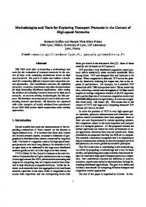
Fig. 1. In Fig. 1, (A) illustrates the distribution of a 1-D Gaussian kernel at four S.D.s, (B) illustrates the zero-th order Gaussian derivative of this kernel as a 2-D grey level image, and (C) as a 3-D wire frame representation.

multiple scales. Consequently, the basic premise of linear scale-space is that a multi-scale representation of a signal (such as a remote sensing image of a landscape) is an ordered set of derived5 signals showing structures at coarser scales that constitute simplifications of corresponding structures at finer scales. In this context, ‘simplification’ refers to smoothed structures resulting from convolution6 with Gaussian kernels of various widths (i.e. scales). In the English literature, the earliest scale-space accounts are attributed to Witkin (1983) who is credited with coining the term, and to the well-developed framework written by Koenderink (1984). Since this time, the Western scale-space community has developed into a serious field of computer vision (Nielsen et al., 1999) with international conferences (ter Haar Romeny, 1997) and several comprehensive published texts (Lindeberg, 1994b; Florack, 1997; Sporring et al., 1997). Yet despite this success, its non-trivial mathematics (i.e. group invariance, differential geometry and tensor anal-

5

Derivatives represent the relationships between the rates of change of continuously varying quantities. The solution of a differential equation is, in general, an algebraic equation expressing the functional dependence of one variable upon one or more others. If, on the other hand, the function depends upon several independent variables, so that its derivatives are partial derivatives, then the differential equation is classed as a partial differential equation. 6 Con6olution involves the passing of a moving window (or kernel) over an image to create a new image where each pixel in the new image is a function of the original pixel values within the moving window and the coefficients of the moving window as specified by the user.

ysis) has limited its adoption outside of computer vision, and until recently (Weickert et al., 1997, 1999; Florack and Kuijper, 1998), cultural differences had obscured the fact that earlier Scale-Space theory and applications were actually pioneered in Japan by Iijima (1959) more than two decades prior to their Western counterparts. It is interesting to note that while early Japanese scale-space research7 was based on determining solutions for optical character recognition, there was also an underlying philosophical motivation behind its evolution. Its principles go back to Zen Buddhism, and may be captured by the phrase ‘Anything is nothing, and nothing is anything.’ This suggests that to obtain the desired information, it is necessary to control the unwanted information. Thus, ‘smoothed’ scale-space structures may be interpreted as a kind of unwanted information, which helps to understand the semantical content of the original image (Weickert et al., 1997).

2.1. Uniqueness of the Gaussian Kernel Gaussian operators (kernels) are fundamental to Scale-Space theory. In one dimension, a Gaussian distribution8-also called a ‘normal distribution’-may be characterized by its familiar ‘bell shaped curve’. In two dimensions, its distribution represents a circular area that radially diffuses

7 Which even today is still considered mathematically elegant and up-to-date (Florack and Kuijper, 1998). 8 For computational reasons, we represent the asymptotic distribution of a Gaussian with four S.D.s (which approximates 99.999% of the theoretical distribution).

32

G.J. Hay et al. / Ecological Modelling 153 (2002) 27–49

outwards from a bright center towards darker edges, while in three dimensions, it appears as a single mountain peak, that grades smoothly to its base (Fig. 1). Their use in Scale-Space theory is not by chance, but instead reflects strict purpose, design, and evaluation. In the following section we discuss these concepts in greater detail. All biological or artificial vision systems require the ability to measure samples from a (real world) scene. This is done through a sampling aperture, which must consist of a finite size in order to integrate the entity to be measured (i.e. light intensity). In an uncommitted framework, there is no information regarding the size to make this aperture, therefore the obvious solution is to leave the aperture size (scale) as a free parameter. In addition, the description of any physical system within an uncommitted framework must be independent of the particular choice of coordinate system, so that if coordinates are changed, the description will still describe the same system. These requirements and others can be stated as axioms, or postulates for an uncommitted visual front end. In essence they represent the mathematical formulation for ‘we know nothing, and we have no preference whatsoever’ (ter Haar Romeny and Florack, 2000). Weickert et al. (1997) provides an overview of more than ten axiomatics for an uncommitted framework that is satisfied by the Gaussian kernel within a linear scale-space framework. In the list below, we describe four of the most important axioms: “ Linearity (i.e. no knowledge, no model, no memory): measurement should proceed in a linear fashion, as non-linearities require the incorporation of a priori knowledge. “ Spatial shift in6ariance (i.e. no preferred location): all scene locations should be measured in the same fashion, i.e. with the same aperture function. “ Isotropy (i.e. no preferred orientation): scene structures with a specific orientation like a horizontal horizon, or vertical trees, should have no measurement preference. This necessitates an aperture with a circular integration area.

“

Scale in6ariance (i.e. no preferred size/scale): any size of structure at this stage of acquisition is just as likely as any other, and there is no reason to acquire information with only the smallest sized apertures. Just as scale represents the free parameter in an uncommitted framework, scale is also the free parameter in biological vision systems. That is, scale is not fixed, but instead is variable. Neuropsychological studies indicate that the retina, and related processing layers, measure input with receptive fields at a wide range of sizes (scales) and at all orientations. The importance of these findings as noted by Young (1985) and Koenderink (1984) is that the receptive fields in the mammalian retina and visual cortex can be well modeled by Gaussian derivatives up to order four. A zero-th order Gaussian kernel is illustrated in Fig. 1B, and a first-order Gaussian derivate and its biological equivalent is illustrated in Fig. 2. For a more explicit description of Gaussian derivative kernels, see Lindeberg (1994a). In this paper, we will deal exclusively with the zero-th order Gaussian derivative. Another important quality is that all partial derivatives of the Gaussian kernel are solutions of the linear, isotropic diffusion equation 9. The diffusion equation describes the physical process that equilibrates concentration differences without creating or destroying mass. This process is governed by well-defined laws relating the rate of flow of the diffusing substance with the concentration gradient causing the flow. Within a scale-space framework, this means that the effect of Gaussian smoothing can be considered as the diffusion gradient of the grey-level intensity of an image over scale (t)10. Thus, not only does the Gaussian kernel and all its partial derivates satisfy the linear diffusion equation, they also exhibit a similarity with biological visual operators, and they satisfy the axioms for an uncommitted vision system,

9 Together with the zero-th order Gaussian, they form a complete family of scaled differential operators. 10 In the diffusion equation, time is the free variable. However, in scale-space, scale is considered equivalent; consequently, scale is represented by (t).

G.J. Hay et al. / Ecological Modelling 153 (2002) 27–49

33

Fig. 2. This figure provides a visual comparison of two Gaussian derivative kernels and their biological equivalents. The top row illustrates how well a first-order Gaussian derivative kernel — shown as a 2-D grey level image (A) and a 3-D wire frame representation (B)-spatially models the measured receptive field sensitivity profile of a cortical simple cell (C). The bottom row illustrates how well the Laplacian of a Gaussian derivative kernel-shown as a 2-D grey level (D) and 3-D wire-frame representation (E)-models the spatial characteristics of a lateral geniculate nucleus (LGN) center-surround cell in the visual cortex (F)11. It is believed that these (2) cells are responsible for vision characteristics related to orientation, position, motion, contrast, color and texture.

namely that of linearity, and no preference for location, orientation and scale. They also represent a family of kernels, where scale-defined as the standard deviation (S.D.) of the Gaussian distribution (t)-is the free parameter (ter Haar Romeny and Florack, 2000). 3. Scale-space methodology part I: generating a multi-scale representation There are two principal components required for any multiscale analysis: the generation of a multi-scale representation, and techniques for feature extraction. In the following section, we outline the methodology for applying scale-space to generate a multi-scale representation from a scanned airphoto, and describe the results.

3.1. The scale-space primal sketch Recall that a linear scale-space representation of a signal (i.e. an image) is an embedding of the 11

As measured by Inter Haar Romeny and Florack, 2000.

original data into a derived one-parameter family of successively smoothed signals that represent the original data at multiple scales. In simple terms, an image is convolved with a Gaussian filter of a specific scale, which results in a derived image. This process is iterated. At each iteration the ‘scale’ of the filter increases (by a fixed amount) resulting in a group of successively smoothed images, each of which are composed of the same grain size and extent. More explicitly, each derived signal (i.e. each new ‘smoothed’ image) is created by convolving the nth-order derivative of a Gaussian (DOG) function with an original signal, where the scale (t) of each derived signal is defined by selecting a different S.D. for the DOG function (at each new iteration). This results in a ‘scale-space cube’, or ‘stack’ of increasingly ‘smoothed’ images that illustrates the evolution of the original image through scale. Each hierarchical layer in a stack represents convolution at a fixed scale, with the smallest scale at the bottom (tmin), and the largest at the top (tmax) (Fig. 3). In practice, a user defines a range of scales, along

34

G.J. Hay et al. / Ecological Modelling 153 (2002) 27–49

Fig. 3. In this figure, the left diagram illustrates the concept of a scale-space cube, or scale-space stack, where individual images have been successively smoothed by convolution with a Gaussian kernel of increasing scale (t) and grouped together. During processing, the spatial resolution and extent of each image remain constant. The smallest t resides on the bottom of the stack; the largest is on the top. In this example, the scale of convolution arbitrarily ranges from t0 (original image) to t100. The right graphic represents the resulting scale-space stack generated by applying linear Scale-Space theory to an image, through scales ranging from t0 – 100.

with a constant scale increment. Thus, (t) is incremented at each iteration by a user-defined constant, where a mathematical function automatically specifies the size of the convolution window (i.e. the number of pixels) necessary to determine the new scale. Witkin (1983), Koenderink (1984) refer to this stack of images as a linear scale-space, while Lindeberg (1993) refers to it as a scale-space primal sketch, because, it bears similarity to the primal sketch proposed by Marr (1982). Marr’s primal sketch represents the most elementary level in a computer-vision framework developed to derive shape information from images. It involves defining primitives consisting of edges, line segments, and blobs, and then grouping these primitives based on their first-order statistics. Appropriately, the main features that arise within any scale-space stack are smooth regions which

are brighter or darker than the background, and which standout from their surrounding. These features are referred to as ‘grey-level blobs’ (Fig. 4).

3.2. Dataset In this paper, linear scale-space is applied to an 8-bit scanned panchromatic airphoto through scales ranging from t0 – 100, with a scale increment of two. Thus the first ‘smoothed’ image in the stack (t1) results from convolving the airphoto (t0) and a Gaussian kernel with a S.D. (i.e. scale) of three, the second smoothed image (t2) with a S.D. of five, etc. These scale variables were chosen based on computational convenience, and the assumption they would provide a representative sample of the multiscale structure inherent within the image/scene. The scanned airphoto has a spa-

G.J. Hay et al. / Ecological Modelling 153 (2002) 27–49

35

Fig. 4. Grey-Level blobs generated from the HSL airphoto (top left). The scale (t) of each image beginning from the top left, to the bottom right is t0,10,20,30,40, respectively. The large inset image is t50.

tial resolution of 2.0 m2, an extent of 500× 500 pixels, and was acquired during the late summer of 1997. Geographically, it represents a portion of the highly fragmented agro-forested landscape typical of the Haut Saint-Laurent region of southwestern Que´ bec. The vegetation in this area is dominated by beech-maple climax forest (Fagus grandifolia Ehrh-Acer saccharum Marsh.) situated on uncultivated moraine islets, with cereal crops grown in the rich lowland marine clay deposits of the Champlain Sea (Meilleur et al., 1994). In this image (Fig. 4), stone hedgerows (dark diagonal linear features) separate bright toned agricultural fields, resulting in rectangular field structures. The high contrast grey-tones of the fields are related to different soil

moisture regimes. Dark tones represent a relatively high content of soil moisture and organics, while bright tones represent increased clay content and reduced soil moisture. The ‘rough’ grey-tone forest-texture (image top) represents a mixed-age deciduous forest resulting from extensive harvesting during the early 19th century (Simard and Bouchard, 1996; Bouchard and Domon, 1997). Large mature deciduous tree crowns dominate the scene, interspersed with early successionnal species. A bright narrow gravel road winds horizontally across the scene segmenting forest and fields. For the remainder of this paper, the stack derived from the Haut Saint-Laurent airphoto will be referred to as the HSL-stack.

36

G.J. Hay et al. / Ecological Modelling 153 (2002) 27–49

Fig. 5. These images have been generated to illustrate the perceptually implicit multiscale structure contained within a linear scale-space representation. They represent a feature enhanced image-set of the HSL-stack at two scale ranges. The top scene ranges from t0 – 100, the bottom scene from t0 – 50. The same orientation, color-table, and opacity level have been applied to each stack. The color palette was developed for visual exploration only.

3.3. Perceptual 6olumetric scale-space structure One of the most unique characteristics of a scale-space primal sketch is the potential to ex-

ploit the spatial association implicit to 2-D greylevel blobs with the perceptual volumetric structures that populate each stack, and which ‘appear’ to link grey-level blobs through scale.

G.J. Hay et al. / Ecological Modelling 153 (2002) 27–49

37

Fig. 6. This figure illustrates four generic blob events and the location of their individual bifurcation events. Circular objects represent binary blobs, while the exterior boundary represents their perceptual structure through scale. Adapted from Lindeberg, 1994a,b.

For example, the two graphics in Fig. 5 illustrate the perceptually implicit multiscale structure contained within the HSL-stack. Specialized ‘inhouse’ color and opacity palettes have been applied at two different ranges of scale, and are intended for visualization purposes only. The upper scene represents scales ranging from t0 – 100, the lower scene from t0 – 50. An important, though subtle concept to appreciate when evaluating these images is that visually distinct volumetric structures of varying sizes and shapes persist only within a specific range of scales, even though smoothing is applied over every part of the image, and through all scales. In addition, it is critical to recognize that, while these illustrations are populated by impressive volumetric structures, they exist perceptually only. That is, there is no topology delineating or relating 2-D structures, i.e., grey-level blobs at a specific scale, to uniquely labeled 3-D objects. To facilitate the description (and eventual quantification) of these perceptual structures we will briefly explain the notion of blob events. To quantify the perceptual structures located within a stack first requires applying feature detectors12 to the grey-level primal sketch (which is discussed in greater detail in Section 4). This results in the generation of simplified geometrical structures that can be linked through scale based on the notion of ‘scale-space events’. A unique 12 (i.e. differential geometry operators composed of Gaussian kernels of different orders).

sub-set of these structures is referred to as blob events, the description of which provides a formal grammar or syntax that we will use to describe the perceptual structures in the HSL-stack. Lindeberg (1993) specifies four generic blob event cases: “ Annihilation— one blob disappears “ Merge— two blobs merge into one “ Split— one blob splits into two “ Creation— one new blob appears It is important to note that while the perceptual structures in the HSL-stack appear as volumes through multiple scales their corresponding blob events are discrete in scale. That is, identifying blob events actually requires defining a single pixel location within a corresponding perceptual volumetric structure. In the literature, this location is referred to as either a ‘bifurcation’ and/or a ‘singularity’ (Fig. 6). For example, in the upper image of Fig. 5, a small ‘floating’ dark blue oval structure, located just to the left of the image center is visible. In the parlance of blob events, the pixel representing the base of this oval structure would be considered the location (x, y) in scale (t) where a unique blob creation bifurcation occurs. Similarly, in both upper and lower images in Fig. 5, numerous arch shaped structures (depicted in light blue tones) represent merge events. The pixel location (x, y, t) where each ‘arm’ of these structures joins to form an arch would be considered a merge bifurcation. When these merge structures are visually evaluated in greater detail, it takes little effort to interpret their evolution through scale as the joining of individual tree crowns into stands, and then into larger forest components.

38

G.J. Hay et al. / Ecological Modelling 153 (2002) 27–49

Fig. 7. This enhanced image-set has been generated to provide further visual exploration of the HSL-stack. Each image-set illustrates a rotated perspective of Fig. 5. The left column represents the range: t0 – 100, the right column represents the range: t0 – 50. Color-tables and opacity have been held constant for each image-set. In A1,2, the right side is illustrated facing forward; in B1,2 the rear view faces forward, and in C1,2 the left side faces forward.

For a more complete evaluation of these and other structures, Fig. 7 provides rotated perspectives of both scenes. Depending on the range of visible scales assessed (i.e. t0 – 50, or t0 – 100), some

‘forest’-merge structures appear to evolve into annihilation events. In both figures, annihilation events also appear as red mound-like structures that spatially coincide with dry-soil areas within

G.J. Hay et al. / Ecological Modelling 153 (2002) 27–49

the agricultural fields. In both figures, split events are less visually obvious. When one considers that this family of perceptually distinct multiscale structures result from diffusive or dissipati6e principles (i.e. Gaussian), it is possible to obtain a clearer appreciation for the concept of hierarchical systems as nearly decomposable systems (Simon, 1962). That is, while distinct hierarchical structures exist as individual image planes or layers in the HSL-stack, the results of the Gaussian filter show how structures interact and diffusively persist through scale, but not through all scales. We also note the impressive vertical structures surrounding high contrast features such as roads, and hedgerows. While it is possible to associate ecological importance to these edges, it is necessary to recognize that one of the limitations of scale-space is that high contrast features tend to persist in scale, regardless of whether or not such features have ecological meaning.

4. Scale-space methodology part II: scale-space-blob feature detection The second component of any multiscale analysis consists of feature detection. Four techniques may typically be applied to a linear scale-space: edge, ridge, corner, and blob detection (Lindeberg, 1996, 1999). While the first three techniques have found useful applications in computer vision, edge detection also represents an active body of research in ecological studies where it is used to evaluate landscape fragmentation and connectedness (Hansen and Di Castri, 1992). An increasingly important body of ecological research also involves developing theory and methods for the detection and linking of dominant scene-structures through scale i.e., image-objects (Hay et al., 2001), or patches (Wu and Levin, 1997). From a scale-space perspective, these dominant scene-structures spatially correspond to significant blobs that have been extracted from a scale-space primal sketch. In the proceeding section, we describe blob-feature detection as introduced by Lindeberg (1993, 1994b)).13 13 In particular, chapters 7 –9 provide an in-depth discussion on the scale-space primal sketch, image-structure, and algorithms for generating scale-space blobs.

39

In some instances, our descriptions do not satisfy the exact order as described by Lindeberg; this is because, we outline how such steps may be computationally achieved. We note that while the following represents a simplified description of a mathematically dense method, even this simplified description is not trivial.

4.1. Step I The first step of scale-space blob detection is to generate the scale-space primal sketch (explained in Section 3). From this, blobs are extracted at all levels of scale. The fundamental objective of scale-space blob detection is to link grey-level blob features at different scales in scale-space to higher order volumetric objects called scale-space blobs, and to extract significant image features based on the level of their appearance and persistence over scales. This is premised on the underlying heuristic that volumetric blob-like structures, which persist in scale-space, are likely candidates to correspond to significant structures in the image/scene. To quantify the qualitative structures illustrated in Figs. 5 and 7, scale-space blobs are first defined using a technique that approximates applying a ‘watershed analysis’ to a grey-scale ‘landscape’.14 To achieve this, 2-D grey-level blobs (Fig. 4) at each scale (t) in the stack are treated as 3-D objects with extent both in space (x, y) and in grey-level intensity (z). Thus, a scale-space blob begins its life with (at least) one local grey-level maxima (i.e. a peak) then analysis proceeds by defining its surrounding region (or watershed). This can be visualized in the following manner. Imagine an image layer from the primal sketch as a flooded 3-D grey-level landscape (Fig. 8). As the water level gradually sinks, peaks will appear. At some instance, two different peaks become connected. The corresponding elevation levels (grey-levels) are called base le6els of the blob. Since these base levels are defined on a 2-D image plane (i.e. an image layer at a specific scale), they repre14 The actual technique involves convolving the 2-D image with the Laplacian of a Gaussian function (see Fig. 2D) at different S.D.s.

40

G.J. Hay et al. / Ecological Modelling 153 (2002) 27–49

Fig. 8. This figure illustrates a single scale (t50) 2-D HSL grey-level blob, represented as a 3-D surface, where z (height) equals the intensity value of each grey-level pixel (vertical exaggeration × 20)

sent unique areas, which define the support region of a grey-le6el blob. “ These areas are converted to a binary mask (i.e. all base level areas are white, the remainder are black) (Fig. 9). “ This process is then applied to each scale (t) of the grey-level stack resulting in corresponding binary blob masks for each scale. “ Each binary mask is then applied to its corresponding grey-level layer, and (z) values are extracted under the mask, resulting in a greyle6el blob layer. “ The extracted z values are integrated to produce a single value that represents the raw grey-level blob volume (x, y, z) for each blob. This is done for each grey-level blob layer.

4.2. Step II The next step is to compute the normalized scale-space volume for each scale-space blob

based on the concepts of effective grey-level blob volume and scale-space lifetime. As blob behavior is strongly dependent upon the structure of the image, this leads one to the conjecture that an expected image beha6ior may exist. To evaluate this, Lindeberg generates greylevel blob volumes from white noise data, i.e. images without any structured relations between adjacent pixels. This is because, when evaluated through scale, even noise has structure (Fig. 10). Therefore, if statistics can be accumulated describing how random noise blobs can be expected to behave in such images, then the result will be an estimate of how accidental blob groupings can be expected to occur in scale-space. If a grey-level blob at some scale has a volume smaller than the expected white-noise volume, then the blob cannot be regarded as significant. Conversely, if at some scale, the blob volume is much larger than the expected volume, and in addition, the difference in blob volume is much greater than the expected variation around the average value, then it is reasonable to treat this blob as significant.

G.J. Hay et al. / Ecological Modelling 153 (2002) 27–49

41

Fig. 9. This figure illustrates defined grey-level blob base le6els (white), which have been converted to binary blobs. The scale (t) of each image, beginning from the top left to the bottom right is t1,10,20,30,40, respectively. The large inset image is t50. The (black) linear features separating each binary blob represent the saddle line, or demarcation zone segmenting two or more different blob (watershed) regions. Mathematically, these lines are composed of zero dimension points; computationally they are composed of single pixels as illustrated.

Based on these considerations, a natural normalization technique is to subtract a measured greylevel blob volume by the mean white-noise grey-level blob volume, and divide by the S.D. of the white-noise grey-level blob volume. This results in a transformed grey-level blob volume. Unfortunately, this value may consist of negative values, making it unsuitable for integration (a necessary step in computing scale-space blob volume). Therefore a value of 1 is added to the transformed 6olume to ensure all positive values. This adjusted value is referred to as the effecti6e grey-le6el blob 6olume.

We note that, for the effective grey-level blob volume to be significantly meaningful, the described mean and S.D. values must represent the results from a large number of stacks (i.e. typically greater than 100) each of which has the same x, y, and t dimensions as the original grey-level stack, and each of which are composed of different white-noise grey-level blob volumes. In several respects, this form of normalization corresponds to the Zen Buddhist reference (see Section 2) that suggests ‘to obtain the desired information, it is necessary to control the unwanted information’.

42

G.J. Hay et al. / Ecological Modelling 153 (2002) 27–49

Fig. 10. Grey-Level blobs generated from a random white-noise image (top left) illustrate that even random noise has structure at different scales. The scale (t) of each image beginning from the top left, to the bottom right is t0,10,20,30,40, respectively. The large inset image is t50. “

“

“

When this normalizing procedure is applied to each layer of raw grey-level blob volumes, it generates normalized scale-space blob volume (6n) layers, which are assembled together in a stack (Sn) corresponding to their associated scales. The corresponding binary blob masks (described in Section 4.1) are also assembled together in a stack (Sb) (Fig. 11). Based on the concepts of blob-events (described Section 3) and scale-space lifetime (described below), binary blobs are then topologically evaluated and labeled as 3-D binary scale-space blob objects— or ‘hyperblobs’.

In essence, the ‘lifetime’ of a scale-space blob is defined by the number of scales between bifurcation events. This concept is central for defining the 4-D topological structure of individual scalespace blobs (Fig. 12). Computationally, we conduct topological linking in a hierarchical manner, where each binary blob at a single layer (tn ) is compared with the binary blobs in the layer above (tn + 1) and below it (tn − 1). If the spatial support of a blob at either upper and or lower levels spatially overlaps the support region of the blobs at (tn ) these blobs are linked through scale, and referred to as a ‘plain link’. If the spatial support of the upper-blob does not overlap the blob at (tn ), an ‘annihilation’ event has occurred. If the

G.J. Hay et al. / Ecological Modelling 153 (2002) 27–49

43

Fig. 11. This figure illustrates a stack composed of binary blobs. For illustrative purposes, each scale of binary blobs has a grey-value associated to it based on its scale of expression. Consequently, the tones grade from dark values at the bottom (t1), to lighter values at the top (t100). The textured base image (t0) is the original airphoto.

spatial support of the lower-blob does not overlap, a ‘creation’ event has occurred at (tn ). If the spatial support of two, or more, upper-blobs overlap then a ‘split’ event has occurred; and if the spatial support of two, or more, lower-blobs overlap then a ‘merge’ event has taken place15. This form of topological linking is applied to all layers in (Sb).16 “ The result is a stack composed of individual hyper-blobs, each of which exhibit a 3-D topology (x, y, t) that explicitly defines their structure and spatial association through scale.

“

“

The individual hyper-blobs are then used as 3-D masks to extract the normalized scalespace volume (x, y, 6n) from each topologically related layer (t) of the normalized blob volume stack (Sn). The extracted (6n) value of each (t) composing individual hyper-blobs is then integrated to produce a single normalized scale-space blob volume (SSbv). This combination of (SSbv) and corresponding hyper-blob structure represent individual 4-D scale-space blobs.

4.3. Steps III and IV 15 This paper outlines the simplest matching relationships between blobs. More sophisticated and computationally complex definitions are provided in Lindeberg, 1994a,b. 16 We note that for topological efficacy, all binary blobs at (tmax) define annihilation events, and all binary blobs at (tmin) define creation events.

The next two procedures involve sorting the resulting scale-space blobs in descending significance order, i.e. with respect to their normalized scale-space blob volumes. Then for each scalespace blob, determining the scale where it assumes

44

G.J. Hay et al. / Ecological Modelling 153 (2002) 27–49

Fig. 12. The graphic on the left represents an imaginary scale-space object (as may be perceived in Fig. 5 Fig. 7) that has been defined by binary blobs in x, y, and t dimensions (shown as stacked grey-level disks). However, this scale-space object exhibits no defined topological relationship with the blobs that perceptually compose it. Conversely, the graphic on the right illustrates how the binary-blobs that compose this perceptual object can be linked (by curved black lines) between bifurcations points (black dots) to define the topological structure of individual Scale-Space blobs. This linking is based on the concepts of scale-space events (see Section 3) and scale-space lifetimes (Ltn ). (A) Represents the bifurcation location of an annihilation event, (M) is the location of a merge event, (S) is a split, and (C) is a creation event. In this graphic, five unique lifetime events are defined (in a bottom up approach). For illustrative purposes the binary-blobs that compose each lifetime are defined with five different shades of grey.

its maximum grey-level blob volume, and extracting the support region of the grey-level blob at this scale. In practice all (SSbv) values are sorted in descending order, resulting in a ranking, where the largest normalized scale-space blob volumes are at the top, the smallest at the bottom. An arbitrary user defined threshold is then applied to define the number of hyper-blobs with the most significant (SSbv) values. From these ‘significant’ hyperblobs, the layer (t) representing the maximum normalized grey-level blob volume (6n(max)) of each hyper-blob is extracted. From this layer, the 2-D spatial support (i.e. corresponding binary blob) is defined and related back to structures in the original image, at the same location. Thus based on the underlying heuristic, 4-D scale-space blobs (x, y, 6n, t) are simplified to normalized 3-D grey-level blobs (x, y, 6n(max)), which are further simplified to their 2-D support region (x, y), and then to the corresponding ‘significant’ objects in the original image.

5. Discussion In this section we discuss the strengths, limitations, and potential ecological applications of Scale-Space theory. We also note the relationship of linear scale-space to wavelets and non-linear Scale-Space theory.

5.1. Strengths In this paper we have suggested that an important limiting factor of the scale-space community has been its highly mathematical nature; ironically, this is also its principal strength. A number of mathematical proofs (Weickert, 1997) state that within the class of linear transformations, the Gaussian kernel is the unique kernel for generating a scale-space representation. It satisfies the solution to the linear diffusion equation. It meets (theoretical) axioms required by an uncommitted vision system, and results from these theoretical considerations are in qualitative agreements with

G.J. Hay et al. / Ecological Modelling 153 (2002) 27–49

results from biological evolution. In addition, the diffusive quality of the Gaussian kernel results in no new structures being added through the scaling process (as occurs with square kernels during convolution); feature detection techniques based on defining edges, ridges, and corners are well documented; and the elegance and utility of being able to evaluate landscape components within a linear scale-specific spatial representation (i.e. a stack) is truly unique. From an analytical perspective, the spatially explicit nature of the ranked 2-D support regions (i.e. binary blobs that result from blob feature detection) can easily be converted for use in GIS, spatial models, and or by spatial statistical packages to be evaluated with landscape metrics (Riitters et al., 1995). From a computational perspective we note that while convolution is efficient with small kernels, processing requirements exponentially increase as kernel sizes (and data set size) increase. To resolve this concern, convolution can be performed in the Fourier domain, where processing is significantly reduced (Ja¨ hne, 1999). In addition, the hierarchical nature of a scale-space primal sketch would lend itself well to automation, multiprocessing and distributed-network solutions, and coding within an object-oriented framework.

5.2. Limitations Generating a linear scale-space stack is not exceptionally difficult once the recipe is understood. The theory is sound, and the processing is relatively straight forward, but blob-feature detection is a non-trivial task, and to the best of our knowledge, no commercially available software exists. ter Haar Romeny and Florack (2000) present a scale-space workbook using the computer algebra package Mathematica, where code for edge, ridge, and corner detection are provided but they do not tackle blob-detection. In this paper, all computer programming has been performed using Interacti6e Data Language (IDL), which has the advantage of processing multidimensional array structures (i.e. 2-D images) essentially in parallel. The remote sensing community is used to discussing scaling in terms of pixel resampling tech-

45

niques (Hay et al., 1997). In Scale-Space theory the pixel size remains constant, yet scaling occurs as the information content of an image is resampled by convolving it with different S.D.s of the Gaussian kernel (i.e. scales) resulting in a stack. While this approach leads to information redundancy, it also allows for the linking of structures through scale. Unfortunately, when applied to a large extent remote sensing data set, significant storage and processing concerns arise. For example, we are currently evaluating scale-space techniques using a high-resolution IKONOS dataset: spatial resolution (grain) is 4 m2 with an extent of 2500× 2500 pixels× 4 spectral channels. Each channel (i.e. image layer) is approximately 15 MB. If we generate a stack with scales ranging from t0 – 100, this represents approximately 1500 MB per stack, for each of the four channels. And when one considers that a minimum of 100 equal sized stacks composed of white-noise grey-level blob volumes also need to be evaluated for each channel (1500 MB× 4×100= 600 GB), the sheer task of computation and storage becomes non-trivial. And this is before any visualization or feature detection occurs. If we strictly obey the axioms of an uncommitted vision system, we need to evaluate a scene at ‘all’ scales. Consequently, a scalespace cube should be composed of (at least) as many pixels in the x, y dimension, as in t, but as suggested, this represents a significant analytical and data representation challenge. From a computational perspective, we note that there are no set rules for determining the maximum number of scales to define within a stack, the increment between these scales, or the threshold number for significance ranking. Another limitation of scale-space is that high contrast features will tend to persist in scale, regardless of whether or not such features have ecological meaning. This also includes the persistence of noise through scale. For further treatment of this subject see Lindeberg (1993) and Starck et al. (1998). In addition, smoothing leads to object shape distortion through scale. We note that while smoothing across ‘object boundaries’ can affect both the shape and the localization of edges in edge detection, this can be resolved by relating different scales of information together.

46

G.J. Hay et al. / Ecological Modelling 153 (2002) 27–49

This is referred to as feature localization (Lindeberg 1999). For example, coarse scale blobs can be identified using coarse scale information, while fine-scale information can be used to further delineate specific structures within the coarse blob boundaries.

5.3. Ecological applications An impressive characteristic of a scale-space primal sketch is the phenomenological, or implicit multidimensional structures that perceptually populate it. When defined, based on the notion of blob-events, they illustrate where and how individual landscape components interact and evolve through scale. Consequently, we suggest that ScaleSpace theory has great potential for improving our understanding of multiscale fragmentation and connectedness in landscapes. In addition, scalespace edge detection has been adapted for treecrown isolation in forestry (Pinz, 1999; Brandtberg and Walter, 1999), and we suggest that it can be further applied for defining the spatial influence of larger landscape-sized objects, i.e. the grain, extent, and location of significant landscape patches. In particular, we have initiated a research program to evaluate the potential of applying the scale-space concept of an uncommitted vision system as a method for defining unbiased landscape structures within high-resolution imagery to fulfill the nondefinitional scaling requirements for hierarchical structures. We are also evaluating how surface interpolation techniques may be applied to bifurcation points—based on their level of appearance— to spatially model critical scale-specific thresholds. We note that non-linear Scale-Space theory is another technique for generating a multiscale representation that is gaining increasing interest in computer vision. The classic paper that began this field in computer vision was by Perona and Malik (1987). Interested readers are also referred to Weickert (1997, 1999) for an overview. In addition, scale-space shares similarities with wavelets; consequently, it can be considered as a special case of a continuous wavelet representation. Interested readers are referred to Lindeberg (1994a,b) and Starck et al. (1998) for a more mathematical description.

6. Conclusion We propose that Scale-Space theory, combined with remote sensing imagery and blob-feature detection techniques, satisfy many of the requirements of an idealized multiscale framework for landscape analysis. Namely, they provide sound mathematical theory and methods to generate a multiscale representation of a scene from a single scale of fine resolution remote sensing data. Significant image features can be automatically defined, and linked through scale based on the level of their appearance and persistence through scales. These spatially explicit image features correspond to ecologically meaningful features within a scene, and their spatial nature allows them to be further evaluated with spatial statistics, or used as inputs in GIS or spatially explicit models. The primary limitations of this framework are that to produce a scale-space stack, a significant amount of ‘redundant’ data needs to be generated. In addition, there are no provided methods or theory describing how to upscale between significantly defined ‘object’ scales17. We envision that with increasing access to multiprocessing distributed networks, the first limitation will diminish. Just as language differences isolated early Japanese and Western scale-space communities, the non-trivial mathematical language used in scale-space formalization also isolates its widespread adoption outside of computer vision by disciplines interested in multiscale theory and methods ranging from biomedical imaging to landscape ecology. The fact that the same body of theory has been developed twice in two very different cultures suggests that it is both natural and noteworthy. Our goal has been to provide an introduction to the theory, methods, and utility of scale-space for exploring and quantifying landscapes within a complex-system framework that is explained without mathematical notation. It is our belief that by providing a non-mathematical primer that consolidates the underlying ideas and theory from classical scale-space papers, that the wealth of the scale-space community will be more 17 Though, we note that this requirement was not part of the original intent of this framework.

G.J. Hay et al. / Ecological Modelling 153 (2002) 27–49

easily accessible, and that new theoretical construct may evolve, and or be adapted by others. The focus of our immediate research lies in two key areas: 1. Evaluating the potential to link the scale-space concept of an uncommitted vision system as a method for defining unbiased landscape structures within high-resolution imagery to fulfill the non-definitional scaling requirements for hierarchical structures. 2. Integrating Complex Systems theory, geostatistics, and 3-D visualization techniques that will allow us to link bifurcation events through space (x, y) and scale (t) so we can evaluate the resulting multiscale surface structures in terms of critical scale-specific landscape thresholds. We hypothesize that these ideas, in concert with the multiscale Object-Specific framework suggested by Hay et al. (2001), and the Hierarchical Patch Dynamics Paradigm of Wu (1999) will bring us closer to understand the processes that lay encoded within multiscale landscape patterns. Acknowledgements This work has been supported by a team grant from FCAR, Gouvernement du Que´ bec, awarded to Dr Andre´ Bouchard and Dr Danielle Marceau, and by a series of scholarships awarded to Hay which include a Bechtel Canada Ph.D. Award of Excellence, a Biology graduate scholarship of excellence from the University of Montre´ al, and a GREFi Ph.D. scholarship (Groupe de recherche en e´ cologie forestie`re interuni6ersitaire). We also thank Frederick Morin for his assistance with coding, and express our appreciation to the organizing and editorial committees for their dedication in ensuring the success of the ‘Modelling Complex Systems: Conference and Workshop’ and this special issue. References Ahl, V., Allen, T.F.H., 1996. Hierarchy Theory: A Vision, Vocabulary, and Epistemology. Columbia University Press, New York.

47

Allen, T.F.H., Starr, T.B., 1982. Hierarchy Perspective for Ecological Complexity. University of Chicago Press, Chicago, p. 310. Allen, T.F.H., Hoekstra, T.W., 1991. Role of heterogeneity in scaling of ecological systems under analysis. In: Kolasa, J., Pickett, S.T.A. (Eds.), In Ecological Studies 86: Ecological Heterogeneity. Springer, pp. 47 – 68. Bak, P., Tang, C., Wiesenfeld, K., 1988. Self-organized criticality. Phys. Rev. A 38, 364 – 374. Bouchard, A., Domon, G., 1997. The transformation of the natural landscapes of the Haut-Saint-Laurent (Que´ bec) and its implication on future resources management. In: Landscape and Urban Planning, vol. 37. Elsevier Science Publ, pp. 99– 107. Brandtberg, T., Walter, F., 1999. An Algorithm for Delineation of Individual Tree Crowns in High Spatial Resolution Aerial Images Using Curved Edges Segments and Multiple Scales. Proceedings of International Forum: Automated Interpretation of High Spatial Resolution Digital Imagery for Forestry. Natural Resources Canada. Canadian Forest Service. Cat. No. Fo42-290/199E pp. 41-54. Coveney, P., Highfield, R., 1991. The Arrow of Time. Flamingo Press, London, p. 378. Florack, L.M.J., 1997. Image Structure. Kluwer Academic Publishers, Dordrecht, The Netherlands. Florack L.M.J., Kuijper, A., 1998. The topological structure of scale-space images. Technical Report UU-CS-1998-31, Department of Computer Science, Utrecht University. Gleick, J., 1987. Chaos. Making A New Science. Penguin Books, p. 352. Hansen, A.J., Di Castri, F., 1992. Landscape Boundaries: Consequences for Biotic Diversity and Ecological Flows. Springer, New York, p. 452. Hay, G.J., Niemann, K.O., Goodenough, D.G., 1997. Spatial thresholds, image-objects, and upscaling: a multiscale evaluation. Remote Sensing Environ. 62, 1 – 19. Hay, G.J., Marceau D.J., Bouchard A., 2001. A Multiscale framework for landscape analysis: object-specific analysis and upscaling. Landscape Ecology 16, 471 – 490. Iijima, T., 1959. Basic theory of pattern observation, Papers of Technical Group on Automata and Automatic Control, IECE, Japan, Dec. (in Japanese) Ja¨ hne, B., 1999. A multiresoluton signal representation. In: Ja¨ hne, B., et al. (Eds.), Handbook on Computer Vision and Applications, vol. 2. Academic Press, Boston, USA, pp. 67– 90. Kay, J., 1991. A non-equilibrium thermodynamic framework for discussing ecosystem integrity. Environ. Manage. 15 (4), 483 – 495. Kay, J., Schneider, E., 1995. Embracing complexity: the challenge of the ecosystem approach. In: Westra, L., Lemons, J. (Eds.), Perspectives on Ecological Integrity. Kluwer, Dodrecht, pp. 49 – 59. Kay. J., Regier, H., 2000. Uncertainty, complexity, and ecological integrity: insights from an ecosystem approach. In: Crabbe, P., Holland, A., Ryszkowski, L., Westra, L. (Eds.), Implementing Ecological Integrity: Restoring Re-

48

G.J. Hay et al. / Ecological Modelling 153 (2002) 27–49

gional and Global Environmental and Human Health, Kluwer, NATO Science Series, Environmental Security pp. 121– 156. Koenderink, J.J., 1984. The structure of images. Biol. Cybernetics 50, 363 – 370. Levin, S.A., 1992. The problem of pattern and scale in ecology. Ecology 73, 1943 –1967. Lindeberg, T., 1993. Detecting salient blob-like image structures and their scales with a scale-space primal sketch: a method for focus-of-attention. Int. J. Comp. Vision 11, 283 – 318. Lindeberg, T., 1994a. Scale-space theory: a basic tool for analysing structures at different scales. J. Appl. Stat. 21 (2), 224 – 270 (Supplement on advances in applied statistics: statistics and images: 2). Lindeberg, T., 1994b. Scale-Space Theory in Computer Vision. Kluwer Academic Publishers, Dordrecht, The Netherlands, p. 423. Lindeberg, T., 1996. Edge detection and ridge detection with automatic scale selection, Technical report ISRN KTH NA/P-96/06-SE. Lindeberg, T., 1999. Principles for Automatic Scale Selection, Technical report ISRN KTH NA/P-98/14-SE. In: Ja¨ hne, B. et al. (Eds.). Handbook on Computer Vision and Applications, vol. 2. Academic Press, Boston, USA pp. 239 –274. Marceau, D.J., 1999. The scale issue in the social and natural sciences. Can. J. Remote Sensing 25, 347 –356. Marceau, D.J., Hay, G.J., 1999. Contributions of remote sensing to the scale issues. Can. J. Remote Sensing 25, 357 – 366. Marr, D., 1982. Vision. Freeman, San Francisco. Meentemeyer, V., 1989. Geographical perspectives of space, time, and scale. Landscape Ecol. 3, 163 –173. Meilleur, A., Bouchard, A., Bergeron, Y., 1994. The relation between geomorphology and forest community types of the Haut-Saint-Laurent, Quebec. Vegetatio 111, 173 –192. Nicolis, G., Prigogine, I., 1977. Self-Organization in Nonequilibrium Systems. From Dissipative Structures to Order Through Fluctuations. Wiley, New York. Nicolis, G., Prigogine, I., 1989. Exploring Complexity: An Introduction. Freeman, p. 313. Nielsen, M., Johansen, P., Olsen, O.F., Weickert, J. (Eds.), 1999. Scale-space theories in computer vision, Lecture Notes in Computer Science, vol. 1682. Springer, Berlin. O’Neill, R.V., King, A.W., 1998. Homage to St. Michael; or, why are there so many books on scale. In: Ecological Scale Theory and Applications. Columbia University Press, pp. 3 –15. Perona, P., Malik, J., 1987. Scale space and edge detection using anisotropic diffusion. In: Proceeding IEEE Computer Society Workshop on Computer Vision (Miami Beach, November 30 to December 2). IEEE Computer Society Press, Washington, pp. 16 – 22. Phillips, J.D., 1999. Divergence, convergence, and self-organization in landscapes. Ann. Assoc. Am. Geographers 89 (3), 466– 488. Pinz, A., 1999. Tree Isolation and Species Classification. Pro-

ceedings of International Forum: Automated Interpretation of High Spatial Resolution Digital Imagery for Forestry. Natural Resources Canada. Canadian Forest Service. Cat. No. Fo42-290/199E pp. 127 – 139. Riitters, K.H., O’Neill, R.V., Hunsaker, C.T., Wickham, J.D., Yankee, D.H., et al., 1995. A factor analysis of landscape pattern and structure metrics. In: Landscape Ecology, vol. 10(1). SPB Academic Publishing BV, Amsterdam, pp. 23 – 39. ter Haar Romeny, B.M., 1997. Applications of scale-space theory. Gaussian Scale-Space Theory. In: Sporring, J., Nielsen, M., Florack, L., Johansen, P. (Eds.), Computational Imaging and Vision. Kluwer Academic Publishers, Dordrecht, pp. 3 – 19. ter Haar Romeny, B.M., Florack, L.M.J., 2000. Front-End Vision, a Multiscale Geometry Engine. Proc. First IEEE International Workshop on Biologically Motivated Computer Vision (BMCV2000), May 15-17, Seoul, Korea. Lecture Notes in Computer Science, Springer, Heidelberg. Saunders, P.T., 1980. An Introduction to Catastrophe Theory Paperback. Cambridge University Pr (Short); ISBN: 0521297826. Schneider, E. 1988. Thermodynamics, information, and evolution: New perspectives on physical and biological evolution. In: B.H. Weber, D.J. Depew & J.D. Smith (Eds.), Entropy, Information, and Evolution: New Perspectives on Physical and Biological Evolution, MIT Press, Boston pp. 10-8 – 138. Simard, H., Bouchard, A., 1996. The precolonial 19th century forest of the Upper St. Lawrence region of Quebec: a record of its exploitation and transformation through notary deeds of wood sales. Can. J. For. Res. 26, 1670 – 1676. Simon, H.A., 1962. The architecture of complexity. Proc. Am. Philosophical. Soc. 106, 467 – 482. Sporring, S., Nielsen, M., Florack:, L., 1997. Gaussian ScaleSpace Theory. Kluwer Academic Publishers, Dordrecht, The Netherlands. Starck, J.-L., Murtagh, F., Bijaoui, A., 1998. Image Processing and Data Analysis: The Multiscale Approach. Cambridge University Press. Urban, D.L., O’Neill, R.V., Shugart, H.H. Jr, 1987. Landscape ecology. A hierarchical perspective can help scientists understand spatial patterns. Bioscience 37 (2), 119 – 127. von Bertalanffy, L. 1976. General System Theory: Foundations, Development, Applications. (Pub) George Braziller. Waldrop, M.M., 1992. Complexity. The emerging science at the edge of order and chaos. Simon and Schuster, p. 380. Watt, A.S., 1947. Pattern and process in the plant community. J. Ecol. 35, 1 – 22. Weickert, J., 1997. A review of nonlinear diffusion filtering. In: ter Haar Romeny, B., Florack, L., Koenderink, J., Viergever, M. (Eds.), Scale-Space Theory in Computer Vision of Lecture Notes in Computer Science, vol. 1252. Springer, pp. 3 – 28. Weickert, J., 1999. Nonlinear diffusion filtering. In: Ja¨ hne, B., et al. (Eds.), Handbook on Computer Vision and Applications, vol. 2. Academic Press, Boston, USA, pp. 423 – 450.

G.J. Hay et al. / Ecological Modelling 153 (2002) 27–49 Weickert, J., Ishikawa, S., Imiya, A., 1997. On the history of Gaussian scale-space axiomatics. In: Sporring, J., Nielsen, M., Florack, L., Johansen, P. (Eds.), Gaussian Scale-Space Theory. Kluwer, Dordrecht, pp. 45 –59. Weickert, J., Ishikawa, S., Imiya, A., 1999. Linear scale-space has first been proposed in Japan. J. Math Imag. Vision 10, 237 – 252. Whittaker, R.H., 1953. A consideration of climax theory: the climax as a population and pattern. Ecol. Monogr. 23, 41 – 78. Wiens, J.A., 1989. Spatial scaling in ecology. Functional Ecol. 3, 385 – 397. Witkin, A.P., 1983. Scale-space filtering. In Proceeding 8th Int.

49

Joint Conf. Art. Intell. (Karlsruhe, Germany), pp. 1019 – 1022. Wu, J., 1999. Hierarchy and scaling: extrapolating information along a scaling ladder. Can. J. Remote Sensing 25, 367 – 380. Wu, J., Levin, S.A., 1997. A patch-based spatial modeling approach: conceptual framework and simulation scheme. Ecol. Modell. 101, 325 – 346. Young, R, 1985. The Gaussian derivative theory of spatial vision: Analysis of cortical cell receptive field line-weighting profiles. Technical Report GMR-4920, General Motors Research.