Oct 5, 1992 - A quantitative test is presented to check scaling and convergence of the correlation integral and consistency of ... Correlation dimensions have been used to inves- ... but the number of peaks in a time series. ... gion of the logarithm of the correlation integral. .... dom can be lower, e.g. if an attractor exists):.
PHYSICS LETTERS A
Physics Letters A 169 (1992) 313—322 North-Holland
A scaling test for correlation dimensions Heinz Isliker InstitutfurAstronomie, ETH Zentrum, CH-8092 Zurich, Switzerland Received 28 October 1991; revised manuscript received 27 May 1992; accepted for publication 5 August 1992 Communicated by A.P. Fordy
A quantitative test is presented to check scaling and convergence of the correlation integral and consistency of two different algorithms. An application to two known attractors demonstrates that it allows one to judge fast and reliably the quality of a conjectured scaling behaviour above all in the case ofshort or noisy data. Results concerning minimum data amount and maximum noise level confirm earlierwork, the crucial parameter concerning data length turns Out, however, to be not the number of points, but the number ofcycles in phase space (peaks in the time series).
I. Introduction Correlation dimensions have been used to investigate whether a process is deterministic or not, However, the last years showed that there is a need for criteria of reliability of dimension estimates. Erroneous dimensions can have two causes: On the one hand, there is a mathematical reason, A class of stochastic processes shows a finite conelation dimension, such as fractional Brownian motion [1]. This motion is approximately a self-similar random path. Self-similarity locally leads to a finite fractal dimension of which correlation dimension is a representative. The dimensions are “erroneous” just in the sense that they are not indicative of deterministic behaviour. Theiler [2] systematically investigates these processes and proposes methods to identify them. On the other hand, erroneous dimensions can result from statistical effects, in three ways: (i) The number of available points might not be sufficient. (ii) The influence of noise is too severe. (iii) There is an uncertainty in identifying a linear scaling region of the logarithm of the correlation integral. The present investigation deals with point (iii) in this second group of error sources. We will present a method to determine the reliability of the linear scaling region in section 3. Applying it in sections 4 and 5 to two well-known examples of attractors of
intermediate dimension (about 2 and 3.5), its efficiency is demonstrated mainly for the case of short or noisy data sets, where the convergence gets worse and worse. As an aside we give reference plots oftypical behaviour ofattractors if the parameter noise and data length are varied. They show that the crucial measure of data length is not the number of points, but the number of peaks in a time series. We start with reviewing two ways of calculating correlation dimensions.
2. Two common ways to determine the correlation dimension According to the time delay method of Takens [3], the phase space is reconstructed from a given a time series {X( t,) } ~ yielding the d-dimensional vectors ~(t,). Different kinds ofdynamical systems yield different kinds of limit sets in state space, so-called attractors, distinguishable by the notion of dimension. For a quasi-periodic motion it is a torus. For a deterministic chaotic process it generally is a complicated invariant set of finite dimension. Finally, a stochastic process is an erratic movement and spans a subset of phase space whose dimension equals the one of the reconstructed state space at least in many cases, compare however the fractional Brownian motion mentioned in the introduction. We resume
0375-960l/92/$ 05.00 © 1992 Elsevier Science Publishers B.V. All rights reserved.
~,
—
313
Volume 169, numberS
PHYSICS LETTERS A
two popular and easily workable definitions of dimension: (A) The Grassberger—Procaccia (GP) method. Grassberger and Procaccia [4] define the correlation integral ~
(e) := urn N-rno
2 N(N—
N
~ 1~~
8(
—
I
—
I)
—
~
3. A measure of reliability of the “plateau” In the GP algorithm, D (2) is usually determined as the linear scaling region in a log ~ (~ )—log e representation, the so-called plateau. How to judge the quality of a plateau? The idea is to use the probabilistic character of the notions: ~ () is a distribution of distances k~(t)—~(t1)I, expected to be of
,
with the Heaviside function 9( ) and any vector norm I. The dimension (2) is defined via C~~,2> (c) ~ correlation 12(2) for a large enough D embedding dimension d. (B) Maximum likelihood (ML) estimate of correlation dimensions [5,6]. The distances j~(t 1)—~(t~) expected to have probability dis2), are with parameter D (2)a This parameter tribution D( can be calculated by means of a maximum likelihood estimate: Assume the scaling law ~~2) to hold for Yi ~ ~ ~ y~.The maximum likelihood formalism yields D (2) =
5 October 1992
n—K ln ( r,
the form ~~(2)~ By means of a f-test it is quantitalively possible to compare the empirical 2~ (c) with the conjectured one 12 (2) distribution checking by C~ that whether it is justified to assume a particular scaling of the correlation integral. Scaling and convergence test. Assume a plateau in the range y~~ ~ y~,suggesting a correlation dimension Then the the test proceeds as follows: (a)~ Divide £-space (space of distances ~(t,) ~(t~) ) into classes, [0, y~]~(Yi (2)] ((2) ~(3)] ((~nd_I) Y2] (4) —
The first class includes the distances smaller than Yi. 1/y2)’
(2)
where the n distances r~:=max(I~(t1)_~(t~)I, ~) are chosen at random, and K denotes the number of distances r2 of equal y~.Elmer shows time that nseries chosen as half the to length of the[6]original yields reasonably accurate results, n = ~ N. (C) Intrinsic error estimate of correlation dimensions. Often, the error of a regression in the log C~2~(e)—log e representation is taken to be the error of the estimated correlation dimension. However, this error is not an intrinsic one. An adequate error estimate, based entirely on the probability interpretation of the notions, is the following [6]: calculating the mean value and the standard deviation of the distribution ~12(2) and propagating the error the Gauss way into D~2~ yields an error 4 ofD~2~ as ______________________
2D(2) l.96D~2~ ~Ji +2 ln(r 2( D(2) D( 2) 12(2) 12(2) (3) 0 )r0 —r0 1 +ln(r~ 4— D( )r 0 —r0 with r 0:=y1/y2, and the factor 1.96 stemming from adopting a 5% confidence interval, as proposed by Ellner.
(b)
Calculate the frequencies of distances
I~(t1)—~(t~)~ in these
classes. Let n~ denote the “empirical” frequency of distances in2~(e), the and kth class, ~~thi) as it “theoretical” is given by the C~ the onedistribution in the same class, calculated from e1~2): 2~((~< c~2~ (c) The test quantity x2 is defined as (~~ X:=
—
~~Ih)
n ~th)
2
(6)
and expected to have a x2 distribution with m~ degrees of freedom. To accept a scaling we demand 1—2
2 satisfies prob[x2~~2]~95%, plateaus with athat toox low significance are rejected. 2~ is estimated Comments. The usedc value of D~ The values from a log C~2~ (e ) —log representation. of e (k) in step (a) can be the values for which the distribution C~2~ () has anyway been evaluated. We generally used 5 ~ m~ 1~ 10.
314
Volume 169, number 5
PHYSICS LETTERS A
This answers the question of goodness of the scaling fit and, by comparing different embedding dimensions, of convergence of the OP algorithm. Consistency. We further demand that the GP value of D (2) is reproduced by the ML algorithm, within the meaningful error 4 of the latter (eq. (3)). This is an intuitive and qualitative criterion. To quantify it we use throughout the upper f-test the value D (2) calculated the ML way. As D (2) is estimated from the same data as the correlation integral, 2 the usual degree of freedom of the x -test is still lowered by one, yielding again m~ 1—2 degrees of freedom. Figure 1 shows a well-behaved case ofconvergence of the GP algorithm for a time series generated with the Mackey—Glass equations (see eq. (11)). It yields a significance of 95% for the marked range, the plateau is accepted. Going to smaller data sets, or increasing the noise level, the quality of the plateau gets worse, and extended numerical experiments with time series generated by different equations (sine wave, Lorenz equations, Rössler equations, Mackey— —
—
5 October 1992
Glass equations) show that even in these well behaved cases the f-test often fails, it does not approve the distinct plateaus. This may partly have numerical reasons, however more important are two theoretical findings: Badii and Politi [7] and Smith et a!. [8] show that for any lacunar set, i.e. a set with sparse regions, the scaling law ~2) cannot hold anymore in a strict sense. It must be replaced by the more general form —
—
2)
(2)
—~
D(
yj(ln/P),
(7)
with w being an unknown periodic function with penod 1: There will generally be superimposed on the plateau an oscillation with completely unknown period and amplitude, both depending on the individual structure of lacunarity. Furthermore, Smith [9] showed that a plateau will be skew, decreasing from its true value at small radii r towards larger radii. A phenomenon caused by the finite size of the attractor: Near the edge, a point is surrounded by other points only on one side. The
15
~10-
-
0
(2
no
~
1” =3.49 ~-8
-6
I
D
,
4
log(o) (400 Cycles) Fig. 1. According to the Grassberger—Procaccia method the slope of the correlation integral log C,~2>(o) against logo is plotted (see eq. (1)) for a time series calculated from the Mackey—Glass equation (eq. (11)). We used 16000 points, the time resolution t was chosen so that ~ 10,- hence the number of cycles ns equals 1600 (see eq. (12)). There is a distinctly flat scaling region for intermediate radii o, modulated by an oscillation towards smaller radii, and by skewness towards larger radii. 315
Volume 169, number 5
PHYSICS LETTERS A
probability distribution for distances, ~j~21, is therefore biased. The typical plateau in fig. 1 for the Mackey—Glass system clearly shows both the above deviation features. The f-test is obviously sensitive enough to detect these oscillating and skew deviations from a wrongly assumed flat scaling region. We are wrong if we expect a behaviour ~2). We do not have access to the true values of the deviations, however we have at least the intrinsic error 4 for the correlation dimension (eq. (3)). It seems therefore reasonable to adjust the f-test, allowing for deviations within the error of the correlation dimension. We propose to use ~~th) max2[ In~n j~th) —
X~dapteci:=
‘~‘I
—‘1k;
0]
(8)
instead off of eq. (6). ‘1k is the error of frequency in the kth class for the distribution ~D(2), due to the error A in D~2~ (eq. (3)): ‘1k
=Z{[(e
(k))D(2)
ln
(k)
2)
ln
1 2 (k_I)]
2} 1/24
(9)
+ [(e (k_i ))D( This allows a plateau to fluctuate between Dt2~—4 and D (2) +4 and to be still acknowledged. Care is to be taken that the frequencies nj,th1) and nj,~°~ are well above the theoretically allowed minimal value of 5. Ifthey are not, the test has a tendency to become too tolerant, the deviations from a plateau it allows for becoming too large. For small numbers of distances imply a large error A (eq. (3)), and by that large tolerances ‘1k. In numerical experiments, this has proven to be a very adequate tool: Slightly oscillating or skew plateaus are still approved. This is illustrated in the next two sections.
4. Application I: the number of points We investigate two intermediately-high-dimensional systems and, with the method of the previous section, we address two problems: How many points are necessaryto detect a correlation dimension, and what is the dependence on the number of points per cycle in phase space? The Rössler attractor, which is the limit set of the three-dimensional Rössler system: —
316
5 October 1992
X= (Y+ Z), Y=X+0.2Y, Z=0.2+Z(X— 5.7) —
(10)
(see ref. [10]). We solved it by a Runge—Kutta algorithm and took the X-coordinate as a time series to analyze fig. 2 shows a part of this time series. — The Mackey—Glass system, whose equation is of the delay type and therefore existing in an infinitedimensional space (the actually used degrees offreedom can be lower, e.g. if an attractor exists): aX( t r) X(t) = 1 + [x(t—rfl10 bX(t) . (11) —
—
We choose a0.2, b=0.1. For a study of this system see ref. [4], whose method of solving the equation is used here, converting the equation into a system of 600 difference equations (for a time profile see fig. 3). Both systems were analyzed in a chaotic regime, using solutionsjust after a certain amount of time to avoid transient correlation features. Thedimensions references values ofthe corresponding were taken from long time series with ten points per cycle in phase space: 16000 points yielded a dimension of 3.49 ±0.17 for the Mackey—Glass attractor; 8000 points in the case of the Rössler attractor showed a dimension of 1.86 ±0.06 (the errors are calculated via eq. (3), with r 0 estimated from the GP procedure and D (2) from the ML procedure). The results are visualized in figs. 4a and 4b for the Rössler and the Mackey—Glass attractor, respectively. The calculations were done in an automatic way, the decision whether there is a plateau or not can be left to the computer a question else becoming awkward for short time series. The user has only to propose ranges Yi 100 13 Havstad and Ehlers [14] find in their numerical experiment an even lower limit for the number of points 319
Volume 169, numberS
PHYSICS LETTERS A
5 October 1992
I’ll’’)
5.0
-
4.5
-
-
I
—
——
-
3.5
-)‘~-=
3.0—
-
I
I
0.000
0.005
The a
I
I
0.010
0.015
of Noise
Fig. 6. Correlation dimension asa function of a, the variance of Gaussian noise added to a time series which is generated by the Mackey— Glass system. The same units are used as in fig. 3. Its length is 4000 points, the time resolution r is chosen so that te,rr/r2 20 and the number of cycles n 5 200. For a> 0.015 the correlation integral did not converge any more.
necessary, using a lot of care in selecting the points on the attractor, however, The quantity n~is also a rough estimate of the number of independent points in phase space, since tcorr is a measure for the duration of dynamical correlation. From theoretical arguments, Smith [9] claims that this number ofindependent points should in order that the dimension fulfill n5~ estimate has an accuracy of 10%. For the Rössler systern (Y2/YI~3.5) this yields ns~250,and for the Mackey—Glass system ns ~ 6500 (where Y2/Yl 2.25). Both numbers are much higher than our empirically found limit of about 100. 21
(5.5Y2/YI)’~
5. Application II: the influence of noise We show how the method is able to recognize plateaus spoilt this time not by shortness, but by noise, Gaussian noise of different variances a was added to the generated time series, in two situations: With the Rössler attractor we looked at the vanation ofthe dimension with the number of structures 320
ns if an intermediate noise level is present (noise to signal ratio between 1% and 10%). Figure 5 presents the result for this attempt, wherethe added noise level is a= 0, i= 0.1 and a= 0.5. The time series has a quite well-defined average amplitude of about 7 (see fig. 2), so that a corresponds to a noise to signal ratio of about 0%, are 1.5% and 7%, respectively. dimension estimates spread around the true The value, with no systematic deviation to be seen, and the fluctuations smaller than 10%. With the Mackey—Glass attractor we increased the noise level for a fixed data length to follow the way how the estimated dimension changes and finally disappears. In fig. 6 is shown how sensitive to noise this attractor is. There is a transition zone for the a’s, where the dimension increases in a smooth way from its reasonable value to higher values. At a=0.0175, the correlation integral did not converge anymore, noise dominates. The noise to signal ratio has no typical values, since the time series shows amplitudes on many quite different scales. For an average amplitude of 0.1, the a= 0.0175 corresponds to a noise level of 17.5%. At a noise level of about l0%,
Volume 169, number 5
PHYSICS LETTERS A
the deviation from the true value of the dimension gets larger than 10%.
6. Conclusions A test of significance of a power law scaling region of the correlation integral is desired to overcome the somewhat subjective part of the method: identifying ( ) —log rea plateau. A regression into the log C~2~ lation would not help for it is always possible and the errors are not meaningful. A test is proposed here that uses the probabilistic character of the correlation integral and determines the significance of a scaling behaviour by a f-test. That the test has to be adapted has strong theoretical reasons. The test is a completion of dimension estimate methods towards being an algorithm, i.e. an automatic proceeding. It is easy to implement, several conjectured scaling ranges can be tested, and their quality can be cornpared. The given applications prove that it is delivering, in the adjusted form, reliable and fast decisions. It efficiently reproduces dimensions with 10% accuracy under the condition that ns ~ 50 or 100, and that the noise level is below 10%. The plots of the applications are also practical references, illustrating typical behaviour of chaotic systems. They lead to the following finding: For small amounts of data the crucial parameter is not the data length but the numben of cycles in phase space (peaks in the time senies). This becomes plausible from the following two considerations: First: A strange attractor is fractal just perpendicular to the trajectories ~( t): Locally, at the point ~(ta), an attractor A looks like the product of a line segment (a piece ~( t) ofthe trajectory) and a fractal set F~( 10) which is perpendicular to the trajectory, F~(,O)J..~(t): A=F~(,0)X~(t)[19]. The dimension of F{(10) can be expected to be the attractor dimension minus one, D (2)_ 1 [20]. Each cycle on the attractor will contribute a point to F{(,0), so that intuitively the fractal structure of this set is the easier detectable, the more cycles there are given; and by that the fractal structure of the attractor as well. Second: The number of structures roughly estimates the number of independent vectors in phase space which can be built from a time series (section 4). Both the two applied dimension estimate meth-
5 October 1992
ods demand that the used vectors are chosen independently. Correlated vectors bias the estimate. Therefore, the number of structures will naturally influence the quality of a dimension estimates more than the number of points in the time series does. Smith [9] investigates conditions on the number of independent vectors. We find the limits he claims to be too high in the investigated cases (section 4). The importance of the number of structures, which is related to the number of independent points in phase space, should be included in theoretical inquiries on the minimum number of necessary data points.
Acknowledgement I would like to thank A.O. Benz and J. Kurths for helpful discussions and criticisms, and H. Scheingraber for passing on to me his experience. This work was supported by the Swiss National Science Foundation (grant No. 2000-5.499).
References [11A.R. Osborne and A. Provenzale, Physica D 35 [21J. Theiler, Phys. Lett. A 155 (1991) 480.
(1989) 357.
[3] F. Takens, in: Lecture notes in mathematics, Vol. 898. Dynamical systemsand turbulence (Springer, Berlin, 1981) ~. 366. [4] P. Grassberger and I. Procaccia, Physica D 9 (1983) 189. [5] F. Takens, in: Lecture notes in mathematics, Vol. 1125. Dynamical systemsand turbulence (Springer, Berlin, 1984) I’ ~ [6] 5. Ellner, Phys. Lett. A 133 (1988)128. [7] R. Badii and A. Politi, Phys. Lett. A 104 (1984) 303. [8] L.A. Smith, J.-D. Fournier and E.A. Spiegel, Phys. Lett. A 114(1986) 465. [9] L.A. Smith, Phys. Lett. A 133 (1988) 283. [10] O.E. Rössler, Phys. Lett. A 57 (1976) 397. [11] J. Kurths and H. Herzel, Physica D 25 (1987) 165. [12] H. Atmanspacher, H. Scheingraber and W. Voges, Phys. Rev. A 37 (1988) 1314. [13] N.B. Abraham, A.M. Albano, B. Das, G. de Guzman, S. Yong, R.S. Gioggia, G.P. Puccioni and J.R. Tredicce, Phys. Lett.A 114 (1986) 217. [14] J.W. Havstad and C.L. Ehlers, Phys. Rev. A 39 (1989) 845. [15]A. Brandstater and H.L. Swinney, Phys. Rev. A 35 (1987) 2207. [16] D. Ruelle, Proc. R. Soc. A 427 (1990) 241.
321
Volume 169, number S
PHYSICS LETTERS A
[17] J. Kurths, A.O. Benz and M.J. Aschwanden, Astron. Astrophys. 248 (1991)270. [18] A.M. Albano, J. Muench, C. Schwartz, A.I. Mees and P.E. Rapp, Phys. Rev. A 38 (1988) 3017.
322
5 October 1992
[19] J.-P. Eckmann and D. Ruelle, Rev. Mod. Phys. 57 (1985) 617. [20] K.J. Falconer, Fractal geometry, mathematical foundations
and applications (Wiley, New York, 1990).