A second-order bundle method to minimize the maximum ... - CiteSeerX

INSTITUT NATIONAL DE RECHERCHE EN INFORMATIQUE ET EN AUTOMATIQUE

A second-order bundle method to minimize the maximum eigenvalue function Franc¸ois Oustry

N ˚ 3738 Juillet 1999 ` THEME 4

ISSN 0249-6399

apport de recherche

A second-order bundle method to minimize the maximum eigenvalue function Fran cois Oustry

Theme 4 | Simulation et optimisation de systemes complexes Projet Numopt Rapport de recherche n3738 | Juillet 1999 | 29 pages

Abstract: In this paper we present a nonsmooth algorithm to minimize the maximum eigenvalue of matrices belonging to an ane subspace of n  n symmetric matrices. We show how a simple bundle method, the approximate eigenvalue method can be used to globalize the second-order method developed by M. L. Overton in the eighties and recently revisited in the framework of the U -Lagrangian theory. With no additional assumption, the resulting algorithm generates a minimizing sequence. A geometrical and constructive proof is given. To prove that quadratic convergence is achieved asymptotically, some strict complementarity and non-degeneracy assumptions are needed. We also introduce a new generation of bundle methods for semide nite programming. Key-words: Eigenvalue optimization, semide nite programming, convex optimization, secondorder bundle methods

(Resume : tsvp)  This work was initiated with a scholarship from ENSTA/DGA (France) and was pursued with a post-doctoral scholarship from INRIA and the NSF grant 655302574100-F1852 at Courant Institute of Mathematical Sciences, New York University, 251 Mercer Street, New York, NY 10012 USA. Revised version submitted to Math. Programming, June 1999. Unit´e de recherche INRIA Rhˆone-Alpes 655, avenue de l’Europe, 38330 MONTBONNOT ST MARTIN (France) T´el´ephone : 04 76 61 52 00 - International: +33 4 76 61 52 00 T´el´ecopie : 04 76 61 52 52 - International: +33 4 76 61 52 52

Une methode de faisceaux du second-ordre pour minimiser la fonction valeur propre maximale Resume : Dans cet article nous presentons une methode d'optimisation non-dierentiable pour

minimiser la valeur propre maximale de matrices symmetriques reelles dependant de maniere ane de parametres reels. Nous montrons comment une methode de faisceaux elementaire, appelee methode des valeurs propres approchees, peut ^etre utilisee pour assurer la convergenve (globale) de l'algorithme du second-ordre propose par M. L. Overton dans les annees 80 et recemment revisite dans le cadre de la theorie du U -Lagrangien. Pour montrer que l'algorithme obtenu produit une suite minimisante, nous utilisons une description geometrique du sous-dierentiel de la valeur propre maximale. Pour garantir une vitesse de convergence quadratique, des hypotheses de stricte complementarite et de non-degenerescence sont requises. En n nous relions notre algorithme avec une classe plus large de methodes de faisceaux, dediees a la programmation sous contraintes de semide nie-positivite.

A second-order bundle method for maximum eigenvalue problems

3

1 Introduction Eigenvalue optimization problems have a long history: as mentioned in [25], Lagrange had already stated in 1773 an eigenvalue optimization problem to design the shape of the strongest axially symmetric column with prescribed length, volume and boundary conditions. Yet it is only very recently that it became an independent area of research with both theoretical and practical aspects. Although the mathematical models of the underlying physical problems are generally not convex, it is notable that the area has very strong connections with convex analysis. In fact, these problems have often a composite structure with a convex component. The role of convex analysis was rst emphasized by R. Bellman and K. Fan in [4]; more recently, this point of view was developed further in [15] and [25]. We consider here a basic eigenvalue optimization problem (P ) inf  (A(x)) x2Rm 1

where 1 (X ) is the largest eigenvalue of X = A(x), element of Sn the space of n  n symmetric matrices and Rm 3 x 7! A(x) := A0 + A x (1) m is ane: A0 2 Sn and A is a linear operator from R to Sn . Existing numerical methods to solve (P ) can be arranged in two classes: interior-point methods and nonsmooth optimization methods. The rst interior-point methods for solving (P ) (in the framework of semide nite programming) were developed by Nesterov and Nemirovski [30]. With the exception of Nemirovski's projective method [31, 26], all the interior-point schemes proposed in the early 1990's (see the numerous references in [5, Chap. II, Notes and References]) were path-following or potential reduction methods. As recently explained in a clear survey by Yu. Nesterov [27], \classical" interiorpoint methods can be seen as a process to transform the initial problem into an equivalent one which can be solved \easily" thanks to an addition of structure: self-concordance is used to obtain the polynomiality of interior-point schemes [31]. A similar presentation can be done for predictorcorrector type methods using small neighborhoods; many variants of them can be found for semide nite programming: to give only a sample we refer to [2, 38, 21]. Our approach is quite dierent but, as we will see, does not exempt us from nding a tradeo between global and local requirements, i.e., between total complexity and speed of convergence. Starting directly from problem (P ) itself, we will use a recent second-order theory, namely the U Lagrangian theory [24], to speed up the asymptotic convergence of a rst-order method developed by Cullum, Donath and Wolfe [6] for a particular instance of (P ) (A diagonal), and by Polak and Wardi [37] in a more general framework. Using the terminology of [16, Chap. XIII], the method can be seen as a Markovian dual bundle method: at each iteration an approximation of the "-subdierential is computed, via a bundling process, without using information from the previous iterations. We call it the approximate eigenvalue method. More recently a stabilization of the cutting planes algorithm was proposed in [39] and enriched in [19, 14, 23, 13] with semide nite models of the objective function; this belongs to the class of primal bundle methods [16, Chap. XV] which are very ecient to solve large-scale problems with a moderate accuracy. When high accuracy is needed, second-order information must be added in the model. Combining a geometrical and the Sequential Quadratic Programming approaches, a local algorithm was presented and analyzed in [10], [34], [36], [35] and [41]; in the latter two papers, a quadratic rate of convergence was obtained. Yet, in this SQP framework, the authors considered only a local analysis; issues of global convergence were not addressed. In this paper, we present, as in [33], the second-order analysis of the maximum eigenvalue function using the U -Lagrangian theory [24] and we show how to use the approximate eigenvalue method to globalize the second-order algorithm while preserving asymptotically a quadratic rate of convergence. Our paper is organized as follows. We rst recall some well-known results on the rst-order analysis of 1 . Then using simple chain rules, we derive easily a rst-order analysis of the composite function RR n3738

4

Francois Oustry

f := 1  A. This enables us to simplify the approximate eigenvalue method developed in x 3: at a point x we consider the enlargement of the subdierential of 1 obtained with eigenvectors associated with "maximal eigenvalues; this set " f (x) plays the role of an approximation of the the true "-subdierential @" f (x). By measuring the quality of this approximation, we provide an explicit "-strategy to ensure global convergence of the method; this is an improvement of [32, Theorem 5.5] where the distance between the exact subdierential of 1 at X 2 Sn and its "-subdierential was considered. In x 4, we present the second-order analysis of 1 using the U -Lagrangian theory. We recall the main result of [33]: this theory provides us with a second-order development of 1 along a smooth manifold: the set Mr of matrices whose largest eigenvalue has multiplicity r. We derive similar results for f with a so-called transversality condition. Then, in x 5, we show how to use the approximate eigenvectors (x 2) to introduce some viscosity in the second-order objects presented in x 4. In particular we provide a constructive characterization of the projection of a matrix X 2 Sn onto the manifold r" (Theorem 5.5). This results in a second-order bundle method which is globally and quadratically convergent. With no additional assumptions, a minimizing sequence is generated. Some strict complementarity and nondegeneracy assumptions are needed to guarantee the quadratic rate of convergence. In x 6 using some duality, we explain how the approximate eigenvalue bundle method is related to a new generation of spectral proximal-type bundle methods in which second-order information can also be introduced. Finally we have chosen a numerical example from combinatorial optimization to illustrate a qualitative distinction between interior-point methods and second-order bundle methods: for the latter methods, superlinear convergence can be observe even when sctrict complementarity does not hold. For the convenience of the reader an appendix explaining the notation is given at the end of the paper.

2 First-order analysis In this section we recall elementary results for the maximum eigenvalue function: the subdierentials of 1 can be characterized as exposed faces of a compact section of the cone of semide nite matrices. Then we propose an enlargement of the subdierential of 1 based on the computation of approximate eigenvectors and a vertical development of 1 , i.e., a development of the function " 7! f"0 (x; d). We derive similar results for f := 1  A using a simple chain rule. This will lead us to the main result of this section: any direction d separating 0 from the chosen enlargement of @f (x) is a \good" descent direction.

2.1 Subdierentials and faces

In this paragraph we give explicit descriptions of the subdierential and the approximate subdierential of 1 . In this analysis, a convex compact set plays a paramount role: the intersection of the cone of semide nite matrices with the hyperplane fV 2 Sn : tr V = 1g,

C n := fV 2 Sn : V  0; tr V = 1g :

(2)

The following result is well-known; the proof is easy to derive via the spectral decomposition of symmetric matrices. Lemma 2.1 The convex set C n is the convex hull of rank-one matrices:

C n = cofqqT : kqk = 1g : Using Rayleigh's variational formulation

1 (X ) =

max

q2Rm;kqk=1

qT Xq ; INRIA

A second-order bundle method for maximum eigenvalue problems

5

together with Lemma 2.1, a support function formulation is obtained: 1 (X ) = C n (X ) : (3) As in [15], we will favor the support function formulation since it will be our main tool in the analysis of x 2.3 . In order to describe the exposed faces of C n (Theorem 2.3), we rst establish the following technical result. Lemma 2.2 Let X and Z be in Sn; let Q = [q1; : : : ; qr ] be an n  r matrix whose columns form an orthonormal basis of ker X . (i) Then, XZ = 0 if and only if there exists Y 2 Sr such that Z = QY QT . (ii) Assume in addition X; Z 2 Sn+ ; then hX; Z i = 0 if and only if there exists Y  0 such that Z = QY QT . Proof. [(i)] We have XZ = 0 if and only if range Z  ker X = span fq1 ; : : : ; qr g. This is equivalent to saying that Z belongs to the subspace span fqi qjT + qj qiT : i; j = 1; : : : ; rg = QSr QT : [(ii)] When X and Z positive semide nite, a consequence of the Schur product Theorem [17, x 5.2] is that tr XZ = 0 if and only if XZ = 0. Then, via (i), Z has the form QY QT ; it is positive semide nite if and only if Y  0. 2 The following theorem recalls previously known geometrical descriptions of @1 (X ) (see [10] or [34]) and, along the lines of [15], makes an explicit link with the exposed faces of C n . Theorem 2.3 (i) Let X 2 Sn and let Q1 be an n  r matrix whose columns form an orthonormal basis of E1 (X ). The face of C n exposed by X is FC n (X ) = fQ1 Y QT1 : Y 2 C r g = cofqqT : kqk = 1; q 2 E1 (X )g ; (4) it is the face exposed by any X 0 2 Sn such that E1 (X 0 ) = E1 (X ). (ii) The subdierential of 1 at X is (5) @1 (X ) = FC n (X ) : Proof. [(i)] Realize rst that (6) cofqqT : kqk = 1; q 2 E1 (X )g = fQ1 Y QT1 : Y 2 C r g : Indeed write any normalized vector of E1 (X ) under the form q = Q1 z , with z 2 Rr and kz k = 1. We get cofqqT : kqk = 1; q 2 E1 (X )g = cofQ1 zz T QT1 : z 2 Rr ; kz k = 1g = Q1 cofzz T : z 2 Rr ; kz k = 1gQT1 ; where, in view of Lemma 2.1, cofzz T : z 2 Rr ; kz k = 1g = C r . Now, by de nition of an exposed face, Z 2 FC n (X ) means Z 2 C n and hX; Z i = C n (X ) = 1 (X ) ; or equivalently, Z 2 C n and h1 (X )In ? X; Z i = 0 : Altogether, (4) is obtained with Lemma 2.2 and FC n (X 0 ) = FC n (X ) if and only if ker (1 (X )In ? X ) = ker (1 (X 0 )In ? X 0 ), i.e., E1 (X ) = E1 (X 0 ). [(ii)] It is well known that the subdierential of a support function C n at a point X is the exposed face of C n exposed by X [16, Example VI.3.1]. 2 The description of the approximate subdierential is also obtained directly from the support function formulation of 1 . RR n3738

6

Francois Oustry

Theorem 2.4 For all "  0, we have

@" 1 (X ) = fZ 2 C n : hZ; X i  1 (X ) ? "g

(7) Proof. The approximate subdierential of a support function is given in [16, Example XI.1.2.5]. Then (7) follows immediately. In [44] the same result is obtained via an analysis of the conjugate function of 1 . 2 The directional derivative of 1 has an easy expression. Theorem 2.5 For all D 2 Sn, we have 01 (X ; D) = 1 (QT1 DQ1 ) : Proof. Use (60) and (5) to obtain 01 (X ; D) = @1 (X ) (D) = maxY 2C r hD; Q1 Y QT1 i = maxY 2C r hQT1 DQ1 ; Y i = 1 (QT1 DQ1 ) : This completes the proof. This result was already established using perturbation theory in [22] and can also be found in [15], [41]. 2 0 It is well-known in nonsmooth optimization that the descent property 1 (X ; D) < 0 of a direction D is unstable, the function X 7! 01 (X ; D) being discontinuous. Minimization algorithms based on this mere property are usually not convergent, because descent along such directions may be numerically insucient. One is much more interested in "-descent directions, for which 01;" (X ; D) := @"1 (X ) (D) is negative. Said otherwise, these directions separate 0 from @" 1 (X ) the continuity of X 7! 01;" (X ; D) [16, Theorem XI.4.1.3] guarantees the numerical eciency of such directions. Yet the diculty here is to get a separation algorithm, and this is the rationale for dual bundle methods [16, XIII,XIV]. This paper follows the same approach; but, instead of separating 0 from @" 1 (X ), we use the structure of our speci c problem to provide a tractable \good approximation" of the latter set.

2.2 Enlargement of the subdierential

Since 1 is the support function of a convex compact set, it can be seen as an in nite-max function. Then a rst idea could be to consider the enlargement proposed in [8, Chap. VI]: the convex hull of the gradients of "-active functions. Here the functions are linear and it is easy to see, via (7), that the obtained enlargement is exactly the "-subdierential of 1 . In [6], J. Cullum, W. E. Donath and P. Wolfe introduced a smaller set: they considered the eigenvectors of eigenvalues at a distance " from 1 (X ) and the convex set generated by the associated rank-one matrices. De nition 2.6 For X 2 Sn and "  0 we de ne  the set of indices of "-largest eigenvalues I"(X ) := fi 2 f1; : : : ; ng : i(X ) > 1 (X ) ? "g ; (8)

 the "-multiplicity of 1(X ) : r" := maxfi : i 2 I"(X )g,  the "- rst eigenspace: E"(X ) := i2I"(X ) Ei(X ), where Ei(X ) is the eigenspace of X associated with the ith eigenvalue i (X ),  its orthogonal complement: F"(X ) := i=2I"(X ) Ei(X ),  the \spectral separation" of ":
"(X ) := r" (X ) ? r" +1(X ).

2

INRIA

A second-order bundle method for maximum eigenvalue problems

7

Pseudospectrum. The notions of approximate eigenvalues can be connected with the recent theory

of pseudospectra of linear operators [43, 42]: this notion is mainly used to cope with the lack of regularity of nonsymmetric matrices; here, for symmetric matrices, a pseudospectrum can also be useful. Indeed it enables us to recover more than rst-order regularity of the largest eigenvalue (precisely some local regularity of the set of approximate subgradients). For a normal matrix (in particular for a symmetric matrix) the "-pseudospectrum comprises the union of the closed balls of radius " about each eigenvalue. In fact we consider here one of these "-balls, the one centered at 1 (X ), and we take its intersection with the spectrum of X . The important role played by the approximate eigenvalues justi es the wording approximate eigenvalues method.

2

Take now an n  r" matrix Q" whose columns form an orthonormal basis of E" (X ). Then we de ne the following compact convex set:

"1 (X ) := cofeeT : kek = 1; e 2 E"(X )g :

(9)

or equivalently, via Theorem 2.3,

"1 (X ) = fQ"Y QT" : Y 2 C r" g = FC n (Q" QT" ) = @1 (Q"QT" ) :

(10)

This set is an outer-approximation of @1 (X ) and an inner-approximation of @" 1 (X ):

Proposition 2.7 Let X 2 Sn. Then for all "  0, we have @1 (X )  "1 (X )  @" 1 (X ) : (11) Proof. The inclusion @1 (X )  " 1 (X ) derives directly from (4) and (9). Another easy inclusion is "1 (X )  C n. Take now Z 2 " 1 (X ): Z = Q"Y QT" with Y 2 C r" implies hZ; X i = hY; QT" AQ"i  r" since

QT" AQ" = diag (1 (X ); : : : ; r" (X ))  r" Ir" and tr Y = 1. Together with (8), we obtain hZ; X i  1 (X ) ? "; since Z 2 C n this means, according to (7), that Z 2 @" 1 (X ). 2

A crucial point consists now in quantifying the (Hausdor) distance between our enlargement and the approximate subdierential. One way to proceed is to get a vertical development of 1 .

2.3 Vertical development

The notion of vertical development is presented in [33]. It will result in Theorem 2.11, which gives an explicit upper bound for the distance between the approximate subdierential and the enlargement "1 (X ). We start with some linear algebra. Lemma 2.8 Let U 2 Rnn be such that U T U = In. Then, there exist n  n matrices (E"; F" ; ; T ) such that 8 the columns of E" are unit vectors of E" (X ) (a) > > > > > (b) < the columns of F" are unit vectors of F" (X )  and T are diagonal and positive semide nite ( c) (12) > > 2 2 >  +T =I (d) > > : U =E +F T (e) " " Proof. In [33, Lemma 5.2], we give a constructive proof of this result for " = 0. There is no diculty to see that the same proof can be applied here by decomposing each column of U on E" (X )  F" (X ) = Rn .

2

The decomposition Rm = E" (X )  F" (X ) provides us with some useful relations.

RR n3738

8

Francois Oustry

Lemma 2.9 Let (E"; F" ; ; T ) be a quadruplet satisfying (12)(a;b;c;d) and  = diag (1; : : : ; n) 2 C n. Then we have,

8 T > E" AF" = F"T AE" = 0 > > <  (X )  hX; (E E T )i   (X ) r" " " 1 T i  r +1 (X ) > h X; F  F " > > : tr (T ) " [tr (T "T )]1=2

(a) (b) (c) (d)

(13)

Proof. [a]: The subspaces E" (X ) and F" (X ) are orthogonal and invariant by X . Then the columns of XF" are in F" (X ) and they to the columns of E" . This implies (a). Ppare orthogonal T T [b]: Since E" E" = i=1 i ei ei , where the ei 's are the columns of E" , we have p X T hX; E" E" i = ieTi Aei : i=1

Now use the fact that for all unit vectors e 2 E" (X ), r" (X )  eT Ae  1 (X ), together with  = diag (1 ; : : : ; n ) 2 C n , to get (b). [c] Similarly to [b], we have

hX; F" F"T i =

p X i=1

ifiT Afi  r" +1 (X )(

n X i=1

i ) = r" +1(X ) :

[d] Note that   In and T is (diagonal) positive semide nite to get tr (T )  tr (T ) :

(14)

Now use  = diag (1 ; : : : ; n ) 2 C n and T = diag (t1 ; : : : ; tn )  0, together with the concavity of the square-root function, to obtain n n X X iti  ( it2i )1=2 : i=1

i=1

In matrix notation, this means tr (T )  [tr (T T )]1=2 . Together with (14), this gives (d). 2 We can now give a key result toward relating the two sets of (7) and (10). Proposition 2.10 Let X 2 Sn, "  0 and   0. For all V 2 @ 1(X ), there exists G" 2 "1 (X ) and ve n  n matrices (E" ; F" ; ; T; ) such that 8 > > > < > > > :

(E" ; F" ; ; T ) satis es (12) (a; b; c; d)  = diag (1 ; : : : ; n ) 2 C n Z = G" + (E" TF"T + F"TE"T ) + (F" T TF"T ? E"T TE"T ) tr T T  r" (X )?r" +1 (X ) =
" 1 (X )

(a) (b) (c) (d)

(15)

Proof. Write the spectral decomposition of Z 2 @ 1 (X ): there exists U 2 Rnn , such that U T U = In and a diagonal matrix  such that Z = U U T . In view of (7), we have  2 C n . Then, apply Lemma 2.8: U = E"+ F" T where (E" ; F" ; ; T ) satis es (12)(a;b;c;d) . Substituting this in the spectral decomposition of Z , we obtain

Z = G" + (E" TF"T + F"T E"T ) + (F" T TF"T ? E"T TE"T ) ; (16) P where G" := E" E"T = pi=1 i ei eTi and the ei 's are unit vectors of E"(X ). According to (10), this means G" 2 " 1 (X ). Then (a; b; c) are satis ed. In order to prove (d), take the scalar product of X

with the left- and right-hand side of (16) and use (13)(a;b;c;d) to obtain

1 (X ) + (r" +1(X ) ? r" (X ))tr (T T )  hX; Z i :

INRIA

9

A second-order bundle method for maximum eigenvalue problems

Since Z 2 @ 1 (X ), we have together with (7), hX; Z i  1 (X ) ? . This enables us to complete the proof. 2 The following result says that " 1 (X ) is a good approximation of @ 1 (X ) for  small enough, depending on the spectral separation of De nition 2.6. Theorem 2.11 For all "  0,   0 and D 2 Sn, we have 01; (A; D)  "1 (X ) (D) + (; ") kDk ; (17) or equivalently, @ 1 (X )  "1 (X ) + B (0; (; ")) ; (18) 2  2  1 = 2 where (; ") := (
" (X ) ) + (
" (X ) ). Proof. Let "  0,   0, D 2 Sn and Z 2 @ 1 (X ). From (15)(c) , we obtain

hZ; Di = hG"; Di + hT; E"T DF" + F"T DE"i + hT T; F"T DF" ? E"T DE"i : Let us bound each of the three terms from above. First, G" 2 " 1 (X ) implies hG"; Di  " 1(X ) (D) :

(19)

Then, denoting (T ) = diag (1 1 t1 ; : : : ; n n tn), we have

hT; E"T DF" + F"T DE"i =

n X i=1

i i ti [hD; ei fiT + fi eTi i] :

p

Now, use the Cauchy-Schwarz inequality, together with kei fiT + fi eTi k = 2, to get p hT; E"T DF" + F"T DE"i  2kDktr (T ) : Similarly we have for the last term hT T; F"T DF" ? E"T DE"i = Pni=1 it2i [hD; fifiT ? eieTi i]  tr (T T ) kDk (kfifiT k + kei eTi k)  2tr (T T ) kDk ; since kfi fiT k = kei eTi k = 1. Putting together (19), (20), (13)-(d) and (21), we get p hZ; Di  " 1(X ) (D) + 2kDk (tr (T T ))1=2 + 2kDk tr (T T ) :

(20) (21) (22)

Together with (15)(d) , we obtain (17); (18) is the geometrical form of (17). 2 We will use this result in a simpli ed form. Corollary 2.12 Let X 2 Sn, "  0 and  2 [0;
"2(X ) ]. Then for all D 2 Sn, we have 01; (X ; D)  "1 (X ) (D) + (
8(X ) )1=2 kDk : (23) " 2 Proof. Since  
"2(X ) , we have 0 
"2(X )  (
"2(X ) )1=2 which, together with (17), gives (23). Finally, we show we have s simple expression for the support function of " 1 (X ): it is the largest eigenvalue of an r"  r" symmetric matrix. Proposition 2.13 Let X 2 Sn. Then for all "  0 and D 2 Sn, we have " 1 (X ) (D) = 1 (QT" DQ") : (24)

Proof. The set " 1 (X ) has the same structure as @1 (X ); the proof is then similar to that of Theorem 2.5. 2 In the following paragraph we extend these results to the composite function f := 1  A. RR n3738

10

Francois Oustry

2.4 Composition with an ane mapping

We recall that A denotes the linear part of A(
) and A its adjoint. First-order composition is based on the following elementary chain rule. Proposition 2.14 For x 2 Rm and "  0,

@" f (x) = A @" 1 (A(x)) :

(25)

Proof. This is a straightforward application of the chain rule given in [16, Theorem XI.3.2.1]. Then an enlargement of @f (x) is the following convex set:

2

"f (x) := A" 1 (A(x)) ;

(26)

f~"0 (x; d) := " f (x) (d) :

(27)

and its associated support function Here we use the notation f~"0 (x; d) to emphasize the analogy with the approximate directional derivative of f at x: f"0 (x; d) := @"f (x) (d) : Applying the linear mapping A in (11), it comes

@f (x)  " f (x)  @"f (x) ; [geometric form] or equivalently

(28)

f 0 (x; d)  f~"0 (x; d)  f"0 (x; d) ; [analytic form]

The quality of this approximation is derived from inequality (23): for all "  0,  2 [0;
" (A(x))] and

d 2 Rm ,

f0 (x; d)  f~"0 (x; d) + (
(8A(x)) )1=2 kA dk  f~"0 (x; d) + (
(8A(x)) )1=2 kdk ; "

"

(29)

where  := supkxk=1 kA(x)k is the largest singular value of A. Furthermore, it is straightforward from (24) and (26) that f~"0 (x; d) is also a maximum eigenvalue: f~"0 (x; d) = 1 (QT" (A d)Q") : (30) In particular for " = 0, we have

f~00 (x; d) = f 0(x; d) = 1 (Q1 (A d)QT1 ) : (31) Ideally we would like to choose " > 0 and nd a so-called direction d of "-descent. Lemma 2.15 ([16, Lemma XIII.1.2.3]) Suppose that d 2 Rm is a direction of "-descent: f"0 (x; d) < 0. Then the set of all t > 0 such that f (x + t d) < f (x) ? " forms a non empty interval. The diculty here is that @" f (x) is so rich that computing its support function f 0 (x; d) for a given direction d or a fortiori looking for the best "-descent direction Argminkdk=1 f 0 (x; d) seems to be as expensive as the original problem (P ). Therefore instead of working with @" f (x) we deal with its inner approximation " f (x). Equality (30) quanti es the eort needed to evaluate f~"0 (x; d): it requires the computation of the largest eigenvalue of an r"  r" matrix. We can now specify to what extent a direction d 2 Rm satisfying at x 2 Rm f~"0 (x; d) < 0 ; (32) is a \good" descent direction.

INRIA

A second-order bundle method for maximum eigenvalue problems

11

Theorem 2.16 Let x 2 Rm , "  0 and d 2 Rm be such that (32) holds. Then (i) d is a direction of (x; ")-descent, where " 0 ~ (x; ") := f"(x;

# d) 2
(A(x)) : " 4kdk

(ii) In addition, assume there exist ! 2 [0; 1],  > 0 and  > 0 such that f~0 (x; d)  ?!kdk2 ;

kdk   and
"(A(x))  ; then

"

(33)

 2 (x; ")  ! 4  :

(34)

2

Proof. It is straightforward from (29).

Remark 2.17 Let g 2 "f (x) be such that d = ?g satis es (33) for ! = 1; then g = proj"f (x) 0. When ! 2]0; 1], g is an approximation of this projection. In x 3.1, we present a separation algorithm

to obtain such directions.

2

3 First-order algorithm We describe here an iterative process to compute -descent directions using the information stored in "f (x),  and " being related as in Theorem 2.16. Then the step-length is determined with a ( nite) dichotomous line-search for -descent. The approximate eigenvalue algorithm and its convergence analysis complete the section.

3.1 Projection problem

The problem we want to solve is

min kgk2 : (35) g2" f (x) This problem is a quadratic optimization problem over the cone of positive semide nite matrices. Indeed, in view of (26) and (10), program (35) is equivalent to 8 > < > :

min kA (Q" Y QT" )k2 Y 0 tr Y = 1 :

(36)

In [35], a similar projection problem is encountered. The authors adopt the following approach: instead of projecting onto " f (x), they project onto a " f (x), i.e., the constraint Y  0 is replaced by Y 2 Sr" . This leads them to a quadratic problem with linear equality constraints which can be solved with classical (and ecient) techniques. Yet this approach has a major drawback: when the minimizer is not positive semide nite, we have no interpretation for the resulting projection; one has to escape from the current iteration and to change the multiplicity r" . Here we compute an approximation g of proj" f (x) 0: we require f~"0 (x; ?g)  ?!kgk2 ; RR n3738

12

Francois Oustry

where ! 2]0; 1] is a tolerance that controls the proximity of g from the projection proj" f (x) 0 (see Remark 2.17). The algorithm we present here is essentially the one proposed by J. Cullum, W.E. Donath and P. Wolfe in [6]. It is an instance of a general scheme, called the support-black box method in [16, x IX.3] to minimize a quadratic form on a convex set. This algorithm is in fact a separation algorithm that was rst exposed in [12]. Nowadays two other alternatives are proposed in the context of proximal type bundle method: one consists in calling an interior-point method subroutine [14] and a more recent one proposes to compute an explicit solution in a well chosen metric [13]. support-black box method Step 0. Set l = 1 and s = s1 2 " f (x).

Step 1. Compute dl = ?projPl 0, where Pl = cofs1 ; : : : ; sl g. Step 2. Compute sl+1 2 " f (x) such that sTl+1 dl = "f (x) (dl ) :

Step 3. (Stopping criterion). If " f (x) (dl )  ?!kdl k2 then STOP. Replace l by l + 1 and return to Step 1.

2

Note that sl+1 in Step 2 has the form A uuT where u is a unit eigenvector associated with 1 (QT" (A dl )Q" ). During the separation process a bundle of "-subgradients fs1 ; : : : ; sk g is generated; in that sense the rst order method presented in this section is a bundle method. The convergence of the support-black box method is investigated in detail in [16, x IX.3]. In particular, we have the following properties. Proposition 3.1 The support-black box method at x 2 Rm with ! 2]0; 1[ converges in a nite number of steps. Assume that the "-Strict Complementarity condition holds at x 2 Rm , proj" f (x) 0 2 ri " f (x) :

(SC )"

Then nite convergence is obtained also if ! = 1. Proof. Set g" := proj" f (x) 0. Then the results are directly derived from Theorem IX.3.3.3 and Proposition IX.3.3.4 in [16]. 2

Remark 3.2 The complexity of the support-black box method is not explicitly known. It seems that the number of steps will depend on the condition number of the linear operator S 3 Y 7! K (Y ) := A(Q Y QT ? 1 (Q QT ) : r"

"

"

"

r"

" "

(37)

Requiring that K" is not singular was already a condition introduced in [35] and was the rst apparition of the notion of transversality in semide nite programming although it was not named as such. The connection is clearly established in [41].

2

3.2 Line-search

Let x 2 Rm and d 2 Rm be produced by the support-black box method of x 3.1, so that f~"0 (x; d) < 0. Then, according to Theorem 2.16, the objective function can be decreased by a positive number (x; "). The problem we consider is now: nd t > 0 such that

f (x + td)  f (x) ? (x; ") :

(38)

INRIA

A second-order bundle method for maximum eigenvalue problems

13

When assumptions of Theorem 2.16 (ii) hold, a simple line-search for -descent can be presented. We expose here a line-search based on a dichotomous scheme controlled by a -descent stopping criterion. For an advanced implementation we refer to [16, Remark XIII.2.1.2]. Line-search

Step 0. Set tL = 0, tR = +1 and t0 = 1. Step 1 (work). Obtain q(t) := f (x + td) and q+0 (t) := f 0(x + td; d) using (31). Step 2 (-descent test). If (38) holds stop. Step 3 (Dichotomous search). If q+0 (t) > 0 set tR := t; else set tL = t. Compute t = tL +2 tR .

2

Theorem 3.3 Let x 2 Rm , " > 0 and d 2 Rm be satisfying the assumptions of Theorem 2.16 (ii). Then the line-search for (x; ")-descent stops after a nite number of steps.

Proof. From Theorem 2.16 (ii), the quantity (x; ") is strictly positive. Use now Theorem 2.16 (i), together with Lemma 2.15: ft :2 R+ : f (x + td)  f (x) ? (x; d)g is a non empty interval. Therefore the dichotomous scheme will detect one of its elements after a nite number of iterations. 2

3.3 The approximate eigenvalues algorithm

To get a simple convergence analysis, the rst-order algorithm we present here will use the following "-strategy (see Figure 3.3). Choose rst a tolerance " > 0. Then de ne at x 2 Rm

X := A(x)

"=n = "(x) r(x) 1 (X )


"(x) (X ) Figure 1: "-strategy 8 > > > > > > > > > > > > < > > > > > > > > > > > > :

R"(x) := fr 2 f1; : : : ; n ? 1g : r (A(x)) ? r+1 (A(x))  n" g ; r(x) :=

(

8 > < "(x) := > :

fr : r 2 min R"(x)g if R"(x) 6= ;

n

otherwise,

f (x) ? r(x) (A(x)) + 2"n if R"(x) 6= ; "

(39)

otherwise.

Here, " is the nal tolerance: Algorithm 3.4 below is aimed at minimizing f within a tolerance ". With reference to De nition 2.6, observe that r(x) is the "(x)-multiplicity of 1 (A(x)). If R"(x) 6= ;, the spectral separation of "(x) is larger than n" . Moreover we have r (A(x)) ? r+1 (A(x)) < n" , for r = 1; : : : ; r(x) ? 1, when r(x) > 1. RR n3738

14

Francois Oustry

Algorithm 3.4

Step 0 (Initialization). Choose the tolerances  > 0, " > 0, ! 2]0; 1[; initialize x := x0 2 Rm . Step 1 (Separation). Set " := "(x) and compute d 2 ?" f (x) satisfying (33) with the support-black box method. Step 2 (Stopping criterion). If kdk   stop. Step 3 (Line-search). Compute t such that

f (x + td)  f (x) ? (x; ") ; with the Safeguarded Armijo Line-Search. Step 5 (Update). Replace x by x + td; return to Step 1.

2

To ensure that our problem (P ) makes sense, we assume that f is bounded from below. We have: Lemma 3.5 The function f is bounded from below if and only if (i) or equivalently, (ii)

0 2 A (C n ) ; (range A)? \ Sn+ 6= f0g :

Proof. From convex duality [16, Chap. X], ?f (0) = inf x2Rm f (x), where f  is the conjugate function of f ; as shown in [44], we have

?f (0) = supfhZ; A0 i : Z 2 C n \ ker Ag : Then f is bounded from below if and only if C n \ ker A = 6 ;, which is clearly equivalent to (i) and (ii). Note that (ii) can be directly obtained from [26]. This leads us to the following result. Lemma 3.6 For all x 2 Rm , the parameter "(x) of (39) is not greater than ". Therefore

"(x) f (x)  @"f (x) :

2

(40)

As a result, if f is bounded from below, we have

(i)
"(x) (A(x))  n" ; (ii) or 0 2 "(x) f (x) :

(41)

Proof. Take x 2 Rm and consider the two following cases. [R"(x) 6= ;]: by construction of "(x) (39), (i) holds:
"(x) (A(x))  n" . Furthermore "(x) = f (x) ? r(x) (A(x)) + 2"n < (r(x) ? 21 ) n"  " ; together with (28) and the fact that the set-valued function " 7! @" f (x) is not decreasing, this gives (40). [R" = ;]: we have r(x) = n and "(x) = ". Hence (40) still holds. Then from (10) and (26), we have "(x) f (x) = A (C n). On the other hand, we know from Lemma 3.5 that f bounded means 0 2 A (C n). This implies (ii). 2

Remark 3.7 In practice we will use " bigger than "(x): at each iteration k we choose "k in [0; maxf"(xk ); k "0 g[ such that
"k (xk ) is maximized, where  2] 21 ; 1[ is a given parameter which forces the convergence of

"k towards ".

INRIA

A second-order bundle method for maximum eigenvalue problems

15

We are now in a position to prove nite convergence of Algorithm 3.4 towards an approximate solution of (P ). Theorem 3.8 Assume that f is bounded from below. Then Algorithm 3.4 stops after a nite number of iterations, yielding x satisfying the approximate minimality condition f (y)  f (x) ? " ? ky ? xk for all y 2 Rm Proof. While kdk > , we have 0 2= "(x) f (x) and according to Lemma 3.6,
"(x) (A(x))  n" . Together 2 " with (34), this gives us f (x) ? f (x + td)  (x; ")  [ m 4 ] n . Then Algorithm 3.4 must stop before N steps, where N is the rst integer satisfying  2 "  ?f  (0) : f (x0 ) ? N m 4 n

2

4 Second-order analysis As with the rst-order analysis, a convenient approach consists in studying the second-order behavior of 1 and then deriving that for the composite function f = 1  A by chain rules. Yet, even though their formulation is simple, chain rules are not easy to obtain here; as explained in [33], we need to introduce a geometrical condition to get them.

4.1 The U -Lagrangian of 1

For a presentation of the U -Lagrangian theory in a more general framework we refer to [24]. The second-order analysis we present here starts with the following idea: consider at X 2 Sn , the largest subspace where 01 (X ;
) is linear. De nition 4.1 At X 2 Sn, we de ne U (X ) := fU 2 Sn : 01(X ; U ) + 01 (X ; ?U ) = 0g ; and V (X ) := U (X )? .

2

The subspaces U (X ) and V (X ) are also characterized as follows. Proposition 4.2 ([24]) Let X 2 Sn. (i) For any G 2 ri @1 (X ), U (X ) and V (X ) are respectively the normal and tangent cones to @1 (X ) at G. (ii) U (X ) and V (X ) are respectively the subspaces orthogonal and parallel to a @1 (X ).

2

A rst attempt to reach second order could consist in introducing the function induced by 1 in U (X ). Yet, proceeding this way we would miss a major fact: a good model of 1 must consider the local behavior of all \active constraints" at X . At this stage geometry can help: it suggests xing the multiplicity (i.e., the \activity") of 1 ; this point of view is the one adopted in [36]. The \surface of activity" is de ned as Mr := fM 2 Sn : 1(M ) = : : : = r (M ) > r+1(M )g : Reference [3] is usually proposed to prove the smoothness of Mr . In fact, it can be obtained as a simple consequence of the Constant Rank Theorem [40, Chap. III x 9]. This gives us a geometrical interpretation of the subspaces U (X ) and V (X ). RR n3738

16

Francois Oustry

Theorem 4.3 ([33, Corollary 4.8]) Let X 2 Mr . The subspaces U (X ) and V (X ) are respectively the tangent and normal spaces to Mr at X : U (X ) = fU 2 Sn : QT1 UQ1 ? 1r (tr QT1 UQ1 )Ir = 0g ; (42) and V (X ) = fQ1 Y QT1 : Y 2 Sr ; hY; Ir i = 0g :

2

The U -Lagrangian is a convex function which identi es locally the \ridge" of 1 . De nition 4.4 Let X 2 Sn and G 2 @1(X ). The U -Lagrangian of 1 at the primal-dual pair (X; G) is the function U (X ) 3 U 7! LU (X; G; U ) := V 2V min(X ) 1 (X + U + V ) ? hG; V i : We de ne also the associated set of minimizers

V (X; G; U ) = ArgminV 2V (X ) 1 (X + U + V ) ? hG; V i :

2

The following theorem is established in [24] for any nite valued convex function, we express it in our speci c context. Theorem 4.5 Let (X; G) 2 Sn  @1 (X ). Then, we have (i) the function LU (X; G;
) is well-de ned and convex over U (X ). Assume, in addition, that G 2 ri @1 (X ). Then, (ii) for all U 2 U (X ), V (X; G; U ) is a nonempty compact convex set which satis es sup

V 2V (X;G;U )

kV k = o(kU k) :

(43)

(iii) In particular, at U = 0, we have V (U ) = f0g, LU (X; G; 0) = 1 (X ) and rLU (X; G; 0) = projU (X ) G exists.

A geometrical interpretation of (43) is that U (X ) is tangent at X to the \ridge":

2

fX + U + V (X; G; U ) : U 2 U (X )g : In our context we can prove that this geometrical set coincides in a neighborhood of X with Mr when G 2 ri @1 (X ). Theorem 4.6 ([33, Theorem 4.11]) Assume (X; G) 2 Sn  ri @1 (X ). Then there exists  > 0 such that, for all U 2 U (X ) \ B (0; ), V (X; G; U ) is a singleton. Moreover the map

U (X ) \ B (0; ) 3 U 7! X + U + V (U ) is a C 1-parameterization of the sub-manifold Mr . This gives us a second-order development of 1 along Mr .

(44)

2

INRIA

A second-order bundle method for maximum eigenvalue problems

17

Theorem 4.7 ([33, Theorem 4.12{Corollary 4.13]) Take (X; G) 2 Snri @1 (X ). Then LU (X; G;
) is C 1 in a neighborhood of U = 0 and we have the following second-order development of 1 1 (X + U + V (U )) = 1 (X ) + hG; U + V (U )i + 21 hr2 LU (X; G; 0)
U; U i + o(kU k2 ) ; where r2 LU (X; G; 0) is known explicitly: r2LU (X; G; 0) = projU (X ) H (X; G) projU (X ) ; and H (X; G) is the symmetric positive semide nite operator

(45)

Sn 3 Y 7! H (X; G) Y := GY [1 (X )In ? X ]y + [1 (X )In ? X ]yY G : The operator r2 LU (X; G; 0) is called the U -Hessian of 1 at (X; G).

2

4.2 Composition with ane operator

When composing with the ane operator A(
), we expect the same type of results as for 1 and we would like to have similar geometrical interpretations. It is obvious that the subspace where f 0 (x;
) is linear and its orthogonal complement can be written:

U f (x) = A?1(U (A(x))) and V f (x) = AV (A(x)) : Yet, when concentrating on second-order, the rst diculty encountered is that the inverse image of Mr , i.e., fx 2 Rm : A(x) 2 Mr g =: Wr ; may be nonsmooth. Then to simplify the analysis, a transversality condition is relevant. De nition 4.8 Transversality We say that A(
) is transversal to Mr at x 2 Wr if and only if (T )

U (A(x)) + range A = Sn : 2

The transversality condition guarantees a one to one relation between @f (x) and @1 (A(x)). Lemma 4.9 Assume that transversality holds at x 2 Rm and take g 2 @f (x). Then there exists a unique G 2 @1 (X ) such that g = A (G); if g is in ri @f (x), G is also in ri @1 (A(x)). Moreover dim V f (x) = r(r2+1) ? 1 ; and dim U f (x) = m + 1 ? r(r2+1) :

(46)

Proof. Apply Theorem 5.5 in [33]: let Q1 be a n  r matrix whose columns form an orthonormal basis of E1 (A(x)); then the mapping V (A(x)) 3 V 7! A(V ) is nonsingular. Together with (42), this implies (46). The one-to-one relation between the subdifferentials is easily derived from the fact that G ? G0 2 V (A(x)) when G and G0 are in @1 (A(x)).

2

Finally transversality is a sucient condition to obtain the dierentiability of the U -Lagrangian of

f and to compute its Hessian via simple chain rules. RR n3738

18

Francois Oustry

Theorem 4.10 ([33, Theorem 5.10]) Assume that the transversality condition holds at x 2 Rm and take g 2 ri @f (x). Then the U -Lagrangian of f at x, U f (x) 3 u 7! LfU (x; g; u) := v2Vmin f (x + u + v) ? gT v ; f (x)

is C 1 in a neighborhood of u = 0. In particular, rLfU (x; g; 0) = projU f (x) g ; and r2 LfU (x; g; 0) = projU f (x) H f (x; G) projU f (x) ; where H f (x; G) := A H (A(x); G) A and G is the unique (via Lemma 4.9) vector of ri @1 (A(x)) such that g = A (G).

2

The operator r2 LfU (x; g; 0) is called the U -Hessian of f at (x; g). The projection operator projU f (x)

is given by the expression [33, Corollary 5.7]: projU f (x) = Im ? K0 (K0 K0 )?1 K0 ; where K0 is obtained by taking " = 0 in (37). The transversality condition enabled M. L. Overton and R.S. Womersley, in [35], to parameterize Mr using exponentials of matrices and to transform the original unconstrained minimization problem into a smooth constrained one. This led them essentially the same second derivative formula. Going along the lines of [35] and [9], we can prove that H (A(x); G) is the second covariant derivative in the Euclidean metric of the function r X 1 ^ 1 (M ) := r i (M ) ; i=1

which is smooth near A(x) 2 Mr and coincides with 1 on Mr . Yet, note that the transversality condition is only sucient to prove the smoothness of LfU (x; g;
). The following example shows us that it is not necessary either to get the dierentiability of LfU (x; g;
) or to guarantee the smoothness of Wr . Example 4.11 Consider the mapping from R2 to S3 de ned by 2 3 x ? x 0 0 1 2 x2 ? x1 0 75 : A(x1 ; x2 ) := 64 0 0 0 1 "

#

We have f (x) = maxfjx1 ? x2 j; 1g and at x^ := 01 the transversality condition does not hold. We " # " # ? 1 ? 1 have obviously @f (^x) = f 1 :  2 [0; 1]g. Then V f (0; 1) = R 1 is unidimensional, whereas the transversality condition would imply, via Lemma 4.9, dim V f (0; 1) = 2. Yet, W2 is linear and therefore smooth in a neighborhood of x^: " # f W2 = x^ + U (x) = x^ + R 11 : Moreover, for all g 2 @f (^x) and u 2 U f (0; 1), v(x; g; u) = f0g and LfU (x; g; u) = 1 is trivially twice dierentiable.

2

INRIA

A second-order bundle method for maximum eigenvalue problems

19

5 Global second-order algorithm

We rst explain how to \stabilize" the U -objects. Then we present the three steps of the global U -Newton algorithm: dual, vertical and tangent steps.

5.1 Enlargement of U

From the enlargement of @1 (X ) introduced in x 2.2, we derive easily an enlargement of U (X ). We give here the "-version of De nition 4.1; note that " 1 (X ) (
) plays the role of 01 (X ;
) = @1 (X ) (
).

De nition 5.1 Let "  0 and X 2 Sn. We de ne U"(X ) as the largest subspace where "1(X ) is linear:

U"(X ) := fU 2 Sn : "1 (X ) (U ) + "1(X ) (?U ) = 0g :

and V"(X ) := U" (X )? .

Proposition 4.2 can also be extended in this context. Proposition 5.2 Let "  0 and X 2 Sn. The subspaces U" and V" are equivalently characterized by: (i) For any G" 2 ri " 1 (X ), U"(X ) and V"(X ) are respectively the normal and tangent cones to " 1 (X ) at G". (ii) U"(X ) and V" (X ) are the subspaces respectively orthogonal and parallel to a " 1 (X ). Proposition 5.6 below will show that U"(X ) is just the usual U at an appropriately shifted matrix X". As a result, all the geometrical interpretations of x 4.1 can be reproduced.

5.2 Dual step

The dual step is essentially done in x 3.1: we compute an approximation of the projection of 0 onto

"f (x) with the support black-box method and obtain g" 2 " f (x) such that f~"0 (x; ?g")  ?!kg"k2 : (47) In fact the support-black box also produces a matrix G" in " 1 (A(x)) such that g" = A (G" ). The subgradient g" will be used to guarantee an ecient descent and the dual variable G" will be needed

to compute the Hessian of the U -Lagrangian. Actually, it is important for quadratic convergence to obtain the exact projection. The following result shows that this is possible. Proposition 5.3 Assume (T ) of De nition 4.8 of and (SC )0 of Proposition 3.1 hold at x 2 Rm . Then for 0 < " <
0 (A(x )) (De nition 2.6) , the "-strict-complementarity condition (SC )" holds in a whole neighborhood of x . Proof. When 0 < " <
0 (A(x )), by continuity of eigenvalues, we have r" (x) = dim E"(A(x)) = r when x 2 B (x ; ) for some  > 0. In fact, for  small enough, we have E" (A(x)) = Etot (A(x)), where Etot (A(x)) is the total eigenspace for the 1 (A(x ))-group at A(x); this notion is de ned in [18] and used in [41, 33]. Then introducing, as in [33, Theorem 4.5], the C 1 map X 7! Qtot (X ) de ned in a neighborhood of A(x ), the projection problem involved in (SC )" can be written together with (10) and (26): min kA (Qtot (A(x))Y Qtot (A(x)T ))k2 : (48) Y 2C r

Then the proof becomes similar to the one of [33, Proposition 6.9].

RR n3738

20

Francois Oustry

 The rst-order optimality conditions of (48) with the transversality condition at x, enable us to use the Implicit Function Theorem and to get a C 1 map B (x ; ) 3 x 7! Y (x) solution of

(48).  The strict complementarity condition at x tells us that Y (x ) is positive de nite.  The continuity of Y (
) implies that Y (x) is positive de nite for x in a neighborhood of x . This means that the "-strict complementarity condition is satis ed in the latter neighborhood.

2

Corollary 5.4 Assume that (T ) and (SC )0 hold at x and take 0 < " <
0(A(x )). Then there exists 1 > 0 such that for all x 2 B (x ; 1 ), the support-black box method with m = 1 produces proj"f (x) 0

in a nite number of steps.

2

Proof. Combine Proposition 3.1 with Proposition 5.3.

5.3 Vertical step

It would be nice to project the current point x onto the manifold Wr := fx 2 Rm : A(x) 2 Mr g. Yet, even in the case where transversality holds, such a projection is very hard to obtain. Nevertheless, in the space of matrices it is easy to compute a point of Mr which satis es the rst-order optimality conditions associated with the projection problem. Consider a spectral decomposition of X 2 Mr :

X = Q""QT" + R"" R"T ; where " and " are respectively r"  r" and (n ? r")  (n ? r") diagonal matrices, and R" is a n  (n ? r") matrix whose columns form an orthonormal basis of E" (X )?. Here the components of " are greater than the components of " . Then de ne for all X 2 Sn ,

^ 1;"(X ) := r1

r" X

" i=1

and

i(X ) ;

X" := ^ 1;"(X )Q" QT" + R""R"T :

We have the following result. Theorem 5.5 The matrix X" satis es the rst-order optimality conditions associated with the projection problem min kM ? X k2 : (49) M 2M r"

Proof. Let M be a solution of (49). From Theorem 4.3, the manifold Mr is smooth in a neighborhood of M and its normal space at M is V (M ). Then the (necessary) optimality conditions associated to (49) at M are M 2 Mr" and X ? M 2 V (M ) : It is obvious that X" 2 Mr" , that X ? X" = Q"[" ? ^ 1;" (X )Ir" ]QT" ;

and that tr (" ? ^ 1;"(X )Ir" ) = 0. This proves X ? X" 2 V (X" ) and completes the proof. We will also use the following property.

2 INRIA

A second-order bundle method for maximum eigenvalue problems

21

Proposition 5.6 Let "  0 and X 2 Sn. We have " 1(X ) = @1 (X" ) U"(X ) = U (X") and V"(X ) = V (X") : Proof. By construction, 1 (X" ) = ^1 " (X ) and E1 (X" ) = E" (X ). Then, together with (10) and (5), we have " 1 (X ) = @1 (X" ). The rest is straightforward. 2 The step (in the space of matrices) from A(x) to A" (x) := [A(x)]" will be called a vertical step or V"-step.

5.4 Tangent step

We assume that, at x 2 Rm , the dual and vertical steps have been previously computed: we have g" (x) = A (G" (x)) 2 " f (x) and A" (x) 2 Mr" . Then we de ne the following quadratic program, 8 > < > :

min hG" (x); U i + 12 hH (A" (x); G" (x)) U; U i U 2 U (A" (x)) A" (x) + U 2 A0 + range (A) ;

(50)

where H is de ned in Theorem 4.7. When G" 2 ri " 1 (A(x)), i.e., (using Proposition 5.6) G" 2 ri @1 (A" (x)), (50) is equivalent to minimizing the second-order approximation of LU (A" (x); G" ;
) subject to A" (x) + U lying in the image of the ane mapping A(
): the existence of a corresponding step in the space of variables is guaranteed. Then, program (50) takes the following form in the space of variables: ( min g" (x)T d + 21 dT H"f (x; G" (x)) d (51) A(x) ? A (x) + A d 2 U (A(x)) "

"

To solve (51), we assume nonemptiness of the feasible domain: there exists d0 2 Rm such that

A(x) ? A"(x) + A d0 2 U"(A(x)) :

(52)

When (52) is feasible, we set u := d ? d0 . Then program (51) amounts to (

min b" (x)T u + 12 uT H f (x; G" (x))u u 2 U"f (x) ;

(53)

where H f is de ned in Theorem 4.10, b" (x) := g" (x)+ H f (x; G" (x)) d0 , and U"f (x) := fu 2 Rm : A u 2 U"(A(x))g. To guarantee that u is well-de ned, we assume that H f (x; G"(x)) is positive de nite. Then, to ensure global convergence, we check whether the direction d := d0 + u satis es f~"0 (x; d)  ?!0 kd2 k ; (54) where !0 is a given number in ]0; ![.

Remark 5.7 Even when applied to a smooth function, global convergence of the Newton algorithm is an open question when the Hessian has an unbounded condition number. This explains the need for an anti-zigzag mechanism, and we found that (54) is useful to prove convergence.

5.5 Global algorithm

The global U -Newton algorithm is organized as follows. RR n3738

22

Francois Oustry

Algorithm 5.8

Step 0 (Initialization). Choose the tolerances  > 0, " > 0, ! 2]0; 1] and !0 2]0; ![; initialize x := x0 2 Rm and set " := "(x). Step 1 (Dual step). Compute g" (x) 2 " f (x) and G"(A(x)) 2 " 1 (A(x)) satisfying (47) using the support-black box method. Step 2 (stopping criterion). If kg" (x)k   stop. Step 3 (Vertical Step). Compute A" (x). Step 4 (Horizontal Step). If (52) is feasible and H f (x; G" (x)) is positive de nite, set d to the solution of (51). If (54) holds and kdk >  go to Step 5. If any of these conditions is not satis ed, set d = ?g" (x). Step 5 (Line-search). Compute t such that f (x + td)  f (x) ? (x; ") ; with the Line-Search of x 3.2. Step 6 (Update). Replace x by x + td and " by "(x + td); return to Step 1.

2

Theorem 5.9 Assume that f is bounded from below. Then Algorithm 5.8 (with m < 1) stops after a nite number of iterations, yielding x satisfying the approximate minimality condition f (y)  f (x) ? " ? ky ? xk for all y 2 Rm :

(55)

Proof. The proof is as in Theorem 3.8, since (54) is guaranteed to hold at each iteration. 2 In order to obtain quadratic convergence, we introduce a condition which can be seen as the generalization of the regularity assumption needed in all Newton-type methods. De nition 5.10 Let x 2 Rm be a solution of (P ). We say that the Strict Second-Order Condition (SSOC) holds at x if (T ) of De nition 4.8 and (SC )0 of Proposition 3.1 hold at x and the U -Hessian of f at (x ; 0) is positive de nite. We rst give consequences of (SSOC ). Proposition 5.11 Assume that x is a solution of (P ) and that (SSOC ) holds at x. Then (i) x is the unique solution of (P ), (ii) for any  > 0 there exists  > 0 such that f (x)  f (x ) +  ) x 2 B (x ; ) ; (iii) for any  > 0 there are " and  small enough, such that Algorithm 5.8 yields at least one iterate in B (x ; ), and all the subsequent iterates remain in B (x ; ) as well. Proof. [(i)]. Decompose an arbitrary d 2 Rm as d = u + v with u 2 U f (x ) and v 2 V f (x ). By de nition of the U -Lagrangian (see Theorem 4.10), f (x + d)  LfU (x ; 0; u). Hence f (x + d)  LfU (x ; 0; u) = f (x ) + 21 uT r2 LfU (x ; 0; 0) u + o(kuk2 ) : If d is small, u is small and clearly f (x + d) > f (x ). [(ii)]. Then argminx2Rm f (x) is bounded; f has bounded level sets ([16, Proposition IV.3.2.5]): say f (x)  f (x0 ) + 1 implies kx ? x k  M . Assume for contradiction that there exist  > 0 and a sequence fxk gk2N such that for k  1, f (xk )  f (x ) + 1  f (x0 ) + 1 and kxk ? x k >  :

k

INRIA

A second-order bundle method for maximum eigenvalue problems

23

Then xk is bounded: kxk ? x k  M . Extract a subsequence converging to some x^ and pass to the limit (using continuity of f ) to obtain the desired contradiction: f (^x)  f (x) and kx^ ? x k >  ; x^ 6= x is a minimizer of f , which contradicts (i). [(iii)]. Observe that Algorithm 5.8 produces a decreasing sequence of f -values: every iterate satis es kx ? xk  M . Given  > 0, take  > 0 as in (ii), set " and  such that " + M  : from (55), at least the nal iterate x satis es f (x)  f (x ) + , hence x 2 B (x ; ); if this occurs before stopping, it occurs at each subsequent iteration. 2  The following lemma will enable us to guarantee that, close enough to a solution x , the exact multiplicity r is identi ed. Lemma 5.12 Assume that 0 < " <
0(A(x )). Then, there exists 2 > 0 such that for all x 2 B (x ; 2 ), r"(x) = r(x) = r ; where r(x) is de ned in (39) and r"(x) := dim E"(x). Proof. When 0 < " <
0 (A(x )), it is clear in (39) that r"(x ) = r(x ) = r . Then, the result derives directly from continuity of all eigenvalues. 2 In the following theorem, we combine Corollary 5.4, Proposition 5.11 and Lemma 5.12 to show that after some iteration Algorithm 5.8 coincides with the U -Newton algorithm presented in [33]. Theorem 5.13 Assume (P ) has a solution x 2 Rm at which (SSOC ) holds. Let Algorithm 5.8 be applied with m = 1 and " > 0,  > 0 and kx0 ? x k suciently small. Assume also that the solution of (51) is accepted by Step 4 and that Step 5 produces t = 1. Then, there exists C > 0 such that kx+ ? xk  C kx ? xk2 : (56) Proof. Consider 1 > 0 of Corollary 5.4 (with " = ") and 2 > 0 of Lemma 5.12. Suppose x0 2 B (x ; ), with 0 <  < minf1 ; 2 g. By Proposition 5.11 (iii), all subsequent iterates are in B (x ; ). Then, from Lemma 5.12, r"(x) = r(x) = r and from Corollary 5.4 the support-black box method with m = 1 converges in a nite number of steps. If in addition, (54) holds and the step length t = 1 is accepted in the line-search, Algorithm 5.8 coincides with the local second order algorithm described in [33]. This algorithm has a quadratic rate of convergence [33, Theorem 6.13]: for  small enough, there exists C > 0 such (56) when x 2 B (x ; ). 2 In the following section we connect this work with recent results on bundle methods for semide nite programming.

6 From dual to proximal-type bundle methods

When presenting the rst-order method in x 3, our main objectives was to provide an algorithm with a simple geometrical description to globalize second-order schemes \a la" Fletcher-Overton. Yet, for practical purposes, the following must be noted: 1. the ratio (use of the information)=(computational cost) in Algorithm 3.4 is pretty low: subgradients and "-subgradients computed during the global process (Step 1) or during the local line-search are used only once, 2. the algorithm is very sensitive to the choice of the "-strategy; choosing at each iteration " = "(x) (39) ensures global convergence but may be not the best policy in practice. Therefore there are advantages to move from a dual Markovian bundle method to a polyhedralsemide nite proximal bundle method [23]. The obtained algorithm, in its rst-order version, is closed to the one described by K.C. Kiwiel in [19] where the precision to compute the largest eigenvalue is also controlled by the global scheme.

RR n3738

24

Francois Oustry

Transporting old subgradients. A rst step consists in using old "-subgradients as "-subgradients at the current point for some "  ". This can be expressed as follows. Proposition 6.1 Let k > 1. Assume that, at each point xi, we have computed gi = AGi 2 "f (xi) with Gi 2 C n for i = 1; : : : ; k ? 1. Let Qk be an n  rk matrix whose columns form an orthonormal basis of E"(A(xk )). Set ~ k := [1 ; : : : ; k?1 ]T 2 Rk?1 , 1k?1 2 Rk?1 the vector of all ones and for "  0 consider the set n ?1 i Gi + Qk Y QT : ~ k 2 Rk?1 ; Y 2 S + Gk;" := Pki=1 rk + k T 1Pk?1~k + hIrk ; Y i = 1; o ?1 i Gi + Qk Y QT ; A(xk )i  f (xk ) ? " : h ki=1 k Then for all "  ", we have "f (xk )  A Gk;"  @" f (xk ) : (57)

Proof. This is a straightforward consequence of (7) and (25). 2 Inclusion (57) suggests that the convex set A Gk;" could be taken as our new approximation of @" f (xk ) at xk .

Using some duality. This leads us to a new projection problem for (35): min kgk2 ; g 2 A Gk;" : P ?1 iGi + Qk Y QTk an element of Gk , the projection Setting Gk := Gk;+1 and denoting by G(~; Y ) := ki=1

problem amounts to

(

min kA GP(~; Y )k2 ; G(~; Y ) 2 Gk (58) ?1 i Gi + Qk Y QT ; A(xk )i ? "  0 : f (xk ) ? h ki=1 k Penalizing the linear inequality constraint by introducing a multiplier 2k > 0, we obtain the new problem (





min kA G(~; Y )k2 + 2k f (xk ) ? (A G(~; Y ))T xk ? hA0 ; G(~; Y )i ? " (59) G(~; Y ) 2 Gk : Now, multiplying the objective function by 1=(2k ) and dropping the constant terms, it is proved in [13, Theorem 11.3.1] that (59) is exactly the dual (in the sense of Lagrangian duality [16, Chap. XII]) of the primal problem min ' (y) + 2k ky ? xk k2 ; y2Rm k where 'k is the mixed polyhedral-semide nite model of f at xk : 'k (y) := Gmax hA(xk ); Gi : 2G k

Recalling the variational formulation of 1 and observing that Gk  " 1 (A(xk )) contains at least one matrix of the form qqT where q is a unit vector in E1 (A(xk )), it is easy to verify that this model satis es 'k (y)  f (y) for all y 2 Rm ; and 'k (yk )  f (yk ) ? " : In this approach the control parameter is (k ) which is updated with a simple strategy [20].

A contribution for large-scale problems The resulting rst-order polyhedral-sdp proximal bundle method seems to be promising to solve large-scale eigenvalue problems: in [23], we present applications from control theory which involve 1000  1000 matrices depending on a large number of decision variables m = 500000.

INRIA

25

A second-order bundle method for maximum eigenvalue problems

7 Dropping strict complementarity: an example from combinatorial optimization In this paragraph we have chosen an example from combinatorial optimization, conceived by Yu. Nesterov [29], to illustrate a qualitative distinction between interior-point methods and second-order bundle methods: for the latter methods, superlinear convergence can be observe even when sctrict complementarity does not hold. This fact seems to be corroborated by the recent theoretical work of A. Forsgren [11]. Let us consider the Boolean quadratic maximization problem ( max xT Qx (BQM ) x 2 f?1; 1gn ; where Q = ?ccT and c = [n ? 1; ?1; : : : ; ?1]. A primal semide nite relaxation [28] for (BQM ) is ( max hQ; X i ; X 2 Sn (SDP ) d(X ) = 1n ; X  0 ; where d(X ) is the diagonal of X . The dual of this problem is then ( min 1Tn u ; u 2 Rn  (SDP ) D(u) ? Q  0 ; where D(u) is the matrix with u1 ; : : : ; un on its diagonal. It is easy to check that the three problems (BQM ), (SDP ) and (SDP ) have the same zero value. The solutions of (BQM ) and (SDP ) are unique: x = 1n and u = 0; X  = 1n 1Tn is a solution of (SDP ). Strict complementarity for (SDP ) [1] does not hold: the matrix D(u ) ? Q + X  = ccT + 1n 1Tn is not positive de nite. Consider now the equivalent eigenvalue formulation of (SDP ) [7, 14]: making the change of variable u = 1n + v with vT 1n = 0, we obtain 8 > < min n  ; (; v) 2 Rn+1 I  Q ? D(v) > Tn : v 1n = 0 ; which is in turn equivalent to the unconstrained eigenvalue problem (EV P ) min v) ; n?1 f (~ v~2R 

P



?1 vi ) . We know that with Rn?1 3 v~ = (v1 ; : : : ; vn?1 ) 7! f (~v) = n 1 Q ? D(v1 ; : : : ; vn?1 ; ? in=1 the notion of strict complementarity (SC )0 in Proposition 3.1 of an eigenvalue problem coincide with the corresponding one in semide nite programing [33, Remark 6.6]. We can verify here by hand that T v~ = 0 and 0 2= ri @f (0): 0 = A ( 1nn1n ) where A is the linear operator

Sn 3 X 7! AX

2 = ?n 64

X11 ? Xnn .. .

X(n?1)(n?1) ? Xnn

3 7 2 Rn?1 ; 5

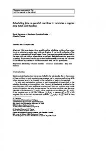
and 1nn1n is in the boundary of @1 (Q). We run Algorithm 5.8 for n = 10 and v~1 = 1n?1 with  = 10?6 , " = 10?4 and ! = 0:1 and v~. Figure 7 can be interpreted as follows: At the initial point the multiplicity is 1 and the distance to the second eigenvalue is large (
"(v~1 ) = 98); therefore the rst-line search is very ecient (recall Theorem 2.16). Yet the descent provokes a clustering of the 9 rst eigenvalues:
"(v~k ) become small but not enough to increase rk := r(~vk ) (39) until iteration 7 where they are counted as n" -eigenvalues. Then second-order steps start to be ecient and superlinear convergence is observed. T

RR n3738

26

Francois Oustry 10

5

0

−5

−10

−15

| Log f (vk ) o rk

−20

−25

−30

−35

1

2

3

4

5 Ieration k

6

7

8

9

Figure 2: Superlinear convergence

8 Conclusion

In this paper, we have shown how to use a second-order theory, the U -Lagrangian theory, to speed up the convergence of a rst-order scheme to minimize the maximum eigenvalue function. The introduction of second-order information in a Markovian dual bundle method (the approximate eigenvalue method of [6, 37]) enabled us to obtain the quadratic convergence of the resulting second-order bundle method when some regularity conditions hold. We also have made a connection with a new generation of bundle methods for semide nite programming.

Acknowledgment

I wish to thank Claude Lemarechal for the numerous and fruitful discussions we had together. I am also greatful to M. Overton for his careful reading and his numerous suggestions to improve the paper. Finally I thank an anonymous referee for his detailed and constructive remarks.

Appendix A Our notation follows closely that of [24] and [15]. Rm m-dimensional Euclidean space xT y scalar p Tproduct of x; y 2 Rm kxk := x x Euclidean norm of x 2 Rm U ? orthogonal subspace of the subspace U projC : Rm ! U projection operator onto the closed convex set C  Rm a C ane hull of the nonempty set C  Rm ri C relative interior of the convex set C  Rm span C linear subspace generated by the nonempty set C  Rm B (x; ) open ball centered at x 2 Rm with radius  > 0 Rm 3 d 7! C (d) := supg2C gT d the support function of the nonempty set C  Rm FC (d) := Argmaxc2C dT c the face of the nonempty set C  Rm exposed by d 2 Rm @f (x) the subdierential of the nite-valued convex function f at x 2 Rm

@f (x) := fs 2 Rm : f (y) ? f (x)  sT (y ? x); for all y 2 Rm g INRIA

A second-order bundle method for maximum eigenvalue problems

27

f 0(x; d) the directional derivative of a convec function f at x 2 Rm in the direction d 2 Rm f 0 (x; d) := t> inf0 f (x + tdt) ? f (x) or equivalently (see [16, x VI.1]), the support function of @f (x) f 0 (x;
) = @f (x) (
)

(60)

@" f (x) the "-subdierential of f at x 2 Rm : @"f (x) := fs 2 Rm : f (y) ? f (x)  hs; y ? xi ? " for all y 2 Rm g f"0 (x; d), the "-directional derivative of f at x 2 R in the direction d 2 R, is the support function of @" f (x): f"0 (x;
) := @" f (x) (
) Sn space of n  n symmetric matrices

Sn+ cone of positive semide nite matrices X  Y (resp. X  Y ) means that the matrix X ? Y 2 Sn is positive de nite (resp. positive

semide nite) P tr X := ni=1 Xii trace of the matrix X 2 Sn hX; Y i :=p tr XY Frobenius scalar product of X; Y 2 Sn kX k := hX; X i Frobenius norm of X 2PSn X y Moore-Penrose inverse of X : if X = ni=1 i (X )qi qiT is the spectral decomposition of X , X y can P be de ned as X y := i (X )6=0 i (1X ) qiqiT 1 (X )  : : :  n(X ) eigenvalues of X 2 Sn in decreasing order E1 (X ) rst eigenspace of X 2 Sn, i.e., the eigenspace associated with 1 (X ) A : Sn ! Rm is the adjoint operator of the linear operator A : Rm ! Sn de ned by: for all (d; D) 2 Rm  Sn hD; A di = dT A D P When A d = mj=1 dj Aj , with Aj 2 Sn for j = 1; : : : ; m, we have for all D 2 Sn , A D = [hA1 ; Di; : : : ; hAm ; Di]T

References [1] F. Alizadeh, J.-P. A. Haeberly, and M. L. Overton. Complementarity and nondegeneracy in semide nite programming. Mathematical Programming, 77:111{128, 1997. [2] F. Alizadeh, J.-P. A. Haeberly, and M. L. Overton. Primal-dual interior-point methods for semide nite programming: Convergence rates, stability and numerical results. SIAM J. Optimization, 8(3):746{768, 1998. [3] V. I. Arnold. On matrices depending on parameters. Russian Math. Surveys, 26:29{43, 1971. [4] R. Bellman and K. Fan. On systems of linear inequalities in Hermitian matrix variables. In V. L. Klee, editor, Convexity, volume 7 of Proceedings of Symposia in Pure Mathematics, pages 1{11. American Mathematical Society, 1963. [5] S. Boyd, L. El Ghaoui, E. Feron, and V. Balakrishnan. Linear Matrix Inequalities in System and Control Theory, volume 15 of Studies in Applied Mathematics. SIAM, Philadelphia, PA, June 1994. [6] J. Cullum, W. E. Donath, and P. Wolfe. The minimization of certain nondierentiable sums of eigenvalues of symmetric matrices. Math. Programming Study, 3:35{55, 1975. [7] C. Delorme and S. Poljak. Laplacian eigenvalues and the maximum cut problem. Mathematical Programming, 62:557{574, 1993. RR n3738

28

Francois Oustry

[8] V.F Demjanov and V.N Malozenov. Introduction to Minimax. Wiley & Sons, 1974. [9] A. Edelman, T. Arias, and S. T. Smith. The geometry of algorithms with orthogonality constraints. Technical report, Massachusetts Institute of Technology, Cambridge, MA 02139, February 1997. Submitted to SIAM J. Matrix. Anal. Appl. [10] R. Fletcher. Semi-de nite matrix constraints in optimization. SIAM J. Control Optim., 23:493{523, 1985. [11] A. Forsgren. Optimality conditions for nonconvex semide nite programming. Technical Report TRITAMAT-1998-OS6, Department of Mathematics, Royal Institute of Technology, 1998. [12] E.G Gilbert. An iterative procedure for computing the minimum of a quadratic form on a convex set. SIAM J. Control, 4:61{80, 1966. [13] C. Helmberg and F. Oustry. Bundle methods to minimize the maximum eigenvalue function. In Lieven Vandenberghe R. Saigal and H. Wolkovicz, editors, Hanbook on Semide nite Programming. Theory, Algorithms and Applications. Kluwer Academic Publisher, 1999. To appear. [14] C. Helmberg and F. Rendl. A spectral bundle method for semide nite programming. Technical Report SC 97-37, Konrad-Zuse-Zentrum fur Informationstechnik Berlin, August 1997. [15] J.-B. Hiriart-Urruty and D. Ye. Sensivity analysis of all eigenvalues of a symmetric matrix. Numerishe Mathematik, 70:45{72, 1995. [16] J.B. Hiriart-Urruty and C. Lemarechal. Convex Analysis and Minimization Algorithms. Springer-Verlag, 1993. Two volumes. [17] R. A. Horn and C. R. Johnson. Topics in Matrix Analysis. Cambridge University Press, 1991. [18] T. Kato. Perturbation Theory for Linear Operators. Springer-Verlag, New York, 1980. [19] K. C. Kiwiel. A linearization algorithm for optimizing control systems subject to singular value inequalities. IEEE Trans. Autom. & Control, AC-31:595{602, 1986. [20] K.C. Kiwiel. Proximity control in bundle methods for convex nondierentiable minimization. Mathematical Programming, 46:105{122, 1990. [21] M. Kojima, M. Shida, and S. Shindoh. Local convergence of predictor-corrector infeasible-interior-point algorithms for sdps and sdlcps. Mathematical Programming, 80:129{161, 1998. [22] P. Lancaster. On eigenvalues of matrices dependent on a parameter. Numerishe Mathematik, 6:377{387, 1964. [23] C. Lemarechal and F. Oustry. Nonsmooth algorithms to solve semide nite programs. In L. El Ghaoui and S-I. Niculescu, editors, Recent Advances on LMI methods in Control, Advances in Design and Control series. SIAM, 1999. To appear. [24] C. Lemarechal, F. Oustry, and C. Sagastizabal. The U -Lagrangian of a convex function. Transactions of the American Mathematical Society, 1997. To appear. [25] A. S. Lewis and M. L. Overton. Eigenvalue optimization. Acta Numerica, 5:149{190, 1996. [26] A. Nemirovsky and P. Gahinet. The projective method for solving linear matrix inequalities. Mathematical Programming, 77:163{190, 1997. [27] Yu. Nesterov. Interior-point methods: An old and new approach to nonlinear programming. Mathematical Programming, 79(1-3):285{297, October 1997. [28] Yu. Nesterov. Quality of semide nite relaxation for nonconvex quadratic optimization. CORE Discussion, Paper # 9719, 1997. [29] Yu Nesterov. Private communication. Center of Operations Research and Econometrics, Universite Catholique de Louvain, B-1348 Louvain-La-Neuve, Belgium, May 1998. [30] Yu. Nesterov and A. Nemirovsky. A general approach to polynomial-time algorithms design for convex programming. Technical report, Centr. Econ. & Math. Inst., USSR Academy of Sciences, Moscow, USSR, 1988. INRIA

A second-order bundle method for maximum eigenvalue problems

29

[31] Yu. Nesterov and A. Nemirovsky. Interior-point polynomial methods in convex programming: Theory and applications, volume 13 of Studies in Applied Mathematics. SIAM, Philadelphia, PA, 1994. [32] F. Oustry. Vertical developments of a convex function. Journal of Convex Analysis, 5(1):153{170, 1998. [33] F. Oustry. The U -Lagrangian of the maximum eigenvalue function. SIAM J. Optimization, 9(2):526{549, 1999. [34] M. L. Overton. Large-scale optimization of eigenvalues. SIAM J. Optimization, pages 88{120, 1992. [35] M. L. Overton and R.S. Womersley. Second derivatives for optimizing eigenvalues of symmetric matrices. SIAM J. Matrix Anal. Appl., 16(3):667{718, July 1995. [36] M. L. Overton and X. Ye. Toward second-order methods for structured nonsmooth optimization. In S. Gomez and J-P. Hennart, editors, Advances in Optimization and Numerical Analysis, pages 97{109. Kluwer Academic Publishers, 1994. [37] E. Polak and Y. Wardi. Nondierentiable optimization algorithm for designing control systems having singular value inequalities. Automatica, 18:267{283, 1982. [38] F. A. Potra and R. Sheng. A superlinearly convergent primal-dual infeasible-interior-point algorithm for semide nite programming. SIAM J. Optimization, 8(4):1007{1028, 1998. [39] H. Schramm and J. Zowe. A version of the bundle idea for minimizing a nonsmooth function: conceptual idea, convergence analysis, numerical results. SIAM J. Optimization, 2:121{152, 1992. [40] L. Schwartz. Cours d'analyse, volume 1. Hermann, Paris, 1967. [41] A. Shapiro and M. K. H Fan. On eigenvalue optimization. SIAM J. Optimization, 5(3):552{568, 1995. [42] Lloyd N. Trefethen. Pseudospectra of linear operators. SIAM Review, 39(3):383{406, 1997. [43] Lloyd N. Trefethen and III David Bau. Numerical Linear Algebra. SIAM, April 1997. [44] D.Y. Ye. Sensitivity analysis of the greatest eigenvalue of a symmetric matrix via the "-subdierential of the associated convex quadratic form. Journal of Optimization Theory and Applications, 76(2), February 1993.

RR n3738

Unit´e de recherche INRIA Lorraine, Technopˆole de Nancy-Brabois, Campus scientifique, ` NANCY 615 rue du Jardin Botanique, BP 101, 54600 VILLERS LES Unit´e de recherche INRIA Rennes, Irisa, Campus universitaire de Beaulieu, 35042 RENNES Cedex Unit´e de recherche INRIA Rhˆone-Alpes, 655, avenue de l’Europe, 38330 MONTBONNOT ST MARTIN Unit´e de recherche INRIA Rocquencourt, Domaine de Voluceau, Rocquencourt, BP 105, 78153 LE CHESNAY Cedex Unit´e de recherche INRIA Sophia-Antipolis, 2004 route des Lucioles, BP 93, 06902 SOPHIA-ANTIPOLIS Cedex

´ Editeur INRIA, Domaine de Voluceau, Rocquencourt, BP 105, 78153 LE CHESNAY Cedex (France) http://www.inria.fr

ISSN 0249-6399