begins when the robot is heading north (0°) after making a right turn at the bottom-left .... top of the figure and then decays rapidly as two wrong turns are made.
A Self-Organizing Temporal Pattern Recognizer with Application to Robot Landmark Recognition Neil R. Euliano & Jose C. Principe Dept. of Electrical Engineering University of Florida Gainesville, FL 32611-2024
Pedro Kulzer Dept. of Electronics and Telecom. University of Aveiro Portugal
Abstract. We propose a new principle that self-organizes an array of processing elements to recognize sequences of input events. The system maps the input onto an output space where the processing elements fire sequentially only when a known pattern is presented. Different input strings will produce unique firing patterns, i.e. the time history is mapped into a spatial pattern. The temporal pattern recognizer is based on the biologically plausible concept of activity diffusion which lowers the threshold of neighboring PEs, thus allowing sequential firing for common patterns. A robotics application is presented where this principle is used to recognize objects from local sensor information.
1. Introduction In most real world applications, the environment which must be learned or understood is temporal in nature. That is, the order of events is often as important as the events themselves. Temporal order is a key feature which enables sophisticated thought processes, language and action. In this paper we present a new temporal pattern recognizer which is trained in an unsupervised fashion (i.e. Self-Organizing). This neural network uses features of the Self-Organizing Feature Map and the key concept of diffusion of activity through time. This diffusion of activity through time lowers the threshold for neighboring neurons after each winner is selected, thus creating a temporally ordered SOFM. We call this network the Self-Organizing Temporal Pattern Recognizer (SOTPAR) and will present its basic features. We also show how the SOTPAR can be used and modified for a landmark recognition task in robotics. The goal is to recognize object shape (a global property) by integrating in time local information obtained through exploration of the object. 2. The SOTPAR Algorithm The methodology presented in this paper creates an array of PEs which selforganizes in space with the help of time information, and can be used for temporal pattern recognition. The system is trains in an unsupervised so that sequences seen during training are mapped into unique spatial sequential firings of the PEs. This produces a discriminant time to space mapping. Discriminant because only known sequences produce an ordered response. Each known sequence produces an
ordered response in a specific area of the output space. The sequential firing facilitates the recognition of temporal patterns by subsequent processing layers. 2.1 Rationale There are three fundamental concepts to the Self-Organizing Temporal Pattern Recognizer [1]: Competitive learning with neighborhood functions, activity diffusion through the space of output PEs, and temporal decay of activations. Using these three concepts, we can convert and distribute the temporal information embedded in the input data into spatial connections and PE distributions in the network, all using self-organizing principles. Similar to Self-Organizing Feature Maps (SOFM), our network uses competitive learning with neighborhood functions [2]. In the SOFM, the input is simultaneously compared to the weights of each PE in the system and the PE which has the closest match between the input and its stored weights is the winner. The winner and its neighbors are then trained in a Hebbian manner, which brings their weights closer to the current input. The key concept in our network is the biologically plausible concept of activity diffusion through the output space. When a PE fires, its activity diffuses to its neighbors and lowers their thresholds, allowing the neighboring PE to be more likely to fire next. We define enhancement as the amount by which this threshold is lowered. If the system is “excitable”, then traveling pulses or wavefronts can be created by the activity diffusion [3]. This wavefront concept is similar to that thought to exist in the dentate gyrus region of the hippocampus, long thought to be the key to short-term memory in the brain [4]. Threshold lowering has been independently done in previous work, but simply on a sample by sample basis, not using the wavefront technique used here [5]. In our model, the local enhancement acts like a traveling wave. This significantly reduces computation of the diffusion equations and provides a mechanism where temporally ordered inputs will trigger spatially ordered outputs. The traveling wave decays over time because of competition for limited resources with other traveling waves. It can only remain strong if spatially neighboring PEs are triggered from temporally ordered inputs, in which case the traveling waves are reinforced. The wavefront enhancement serves the very important function of including context into the winner selection process. The past history of the input signal is stored in the spatio-temporal activity of the 0.3 wavefronts. If this history is a known 0.25 sequence, then the network responds with a 0.2 large wavefront. This wavefront can be 0.15 thought of as focusing the attention of the network on a certain area of the output map 0.1 based on the context – thus improving the 0.05 10 recognition of noisy sequences. Figure 1 0 5 0 -2 shows the memory kernel for the SOTPAR -4 -6 -8 -10 0 PE Number Time system. This figure represents the contribution to the context from each node in Figure 1 - Spatio-Temporal a 1-D system over time. Memory Kernel for SOTPAR The last concept in our algorithm is the
decay of output activation over time. This is also biologically plausible [6] and allows for the temporal wavefront to spread outwards over time. This spreading creates a more robust architecture which can gracefully handle both time-warping and missed or noisy data points. The decay of activity from past inputs is also a biologically plausible explanation for neighborhood threshold lowering. 2.2 Algorithm Description To simplify the description of the algorithm, we will use one-dimensional neighborhoods in 2D maps. We also choose to let the activity propagate in only one direction since the movement of the activity is severely restricted 1-u 1-u 1-u in the one-dimensional case. Thus, the output space consists of strings mem u mem u mem of PEs where each PE has its own weights. The activity/enhancement moves in the direction of increasing PE 1 PE 2 PE 3 PE number and decays at each step. A typical array of PEs is shown in Figure 2. The factors u and (1-u) input are used to normalize the total data 2D Input activity in the network. The parameter u links the activity decay Figure 2 - Typical Array of PEs at each node to the wavefront decay. If u is near 1, the activity at each node is an impulse and the wavefront is restricted to moving one step for every input. If u is near 0, the wavefront activity is very small and the PEs are likely to fire repeatedly for successive inputs. In our simulations, the values of u between 0.5 and 0.7 provide reasonable results. This activity diffusion mechanism serves to store the temporal information in the network. Through training, the PEs will be spatially ordered to sequentially follow any temporal sequences presented. The activity input is a thresholded and enhanced version of the actual SOFM activity. The activity of the network at each iteration is determined by calculating the distance (or dot product) between the input and the weights of each PE and allowing for membrane potential decay: act (t , x ) = act ( t − 1, x ) *(1 − u) + dist ( inp( t ), w x ) *( u ) where act(t,x) represents the activity at PE x at time t, and dist(inp(t),wx) represents the distance between the input at time t and the weights of PE x. A simple threshold and enhancement can be implemented as follows before being propagated: act ′ ( x ) = max( act ( x ) −.5,0) * 2 Next, the winning PE is selected by winner = arg max( act ( x ) + β * enhancement ( x )) x
where the enhancement is the activity being propagated from the left. The parameter β is the spatio-temporal parameter which determines the amount that a temporal wavefront can lower the threshold for PE firing. As β 0, the system operates like a standard SOFM and when β ∞ the system operates like an avalanche network [7]. In other words, β determines the amount of contextual
Æ
Æ
information used in the selection of the winning node. Once the winner is selected, the training is identical to the standard SOFM algorithm. In our current implementation, the spatio-temporal parameter, the learning rate, and neighborhood size are all linearly annealed for better convergence. More extensive discussions and examples of the SOTPAR can be found in reference [1]. 3. Landmark Discrimination and Recognition 3.1 Problem Description In lieu of complicated vision systems, simple robots must use intelligent recognition systems to determine location and navigation. Our robot has only forward and lateral infrared sensors with a narrow field-of-view (~10°) which can detect only if it is near on object. There is no long distance vision or perspective obtained by these sensors, simply an input which detects objects in the 3 lines-ofsight (ahead, left, and right). The robot must navigate through its environment which consists of object landmarks. The landmarks are of various shapes and the robot must use its “inertial navigation system” (a compass and a shaft encoder on the stepper motor) and the landmarks it finds in its environment for proper navigation. Our robot uses wall-following techniques (similar to a blind person who can only feel the walls of a building) to determine the shape of the landmark. Using the limited information obtained by the shaft encoder and object detection sensors, the robot must discriminate between different landmark shapes while it traverses the walls of an object/landmark. After finding a landmark, the robot starts wall-following, trying to keep a fixed distance from it using its front and lateral sensors. The main limitation of this technique is that the circumvention and corner detection will tend to be imprecise. To achieve better cornering and more precise movement, the speed of the robot would be severely limited. The robot circumvents the object by moving a fixed distance between turns, then determining which sensors still detect walls in order to make the next turn. The data that will be collected as the robot traverses the landmark will simply be a string of turn angles and compass headings at equally spaced distances (as determined by the shaft encoder). The relative coordinate turn angle is the derivative of the compass setting and thus this creates a dynamic state-space description of the motion of the robot. If a compass is not present, the turn angle can be derived from the wheel motions and the compass would be the integral of the turns, but the compass would drift over time and would soon be unusable. The main difficulties with this application are: • the exact location where the robot first encounters the landmark is unknown • the circumference of the object is unknown (how do you know when you have traversed it completely) • the robot would like to learn the landmarks very quickly, preferably in a single circumvention • the data collected will be noisy due to the sloppy turns
To help in the recognition of objects from any starting position, we subsample (by 5) the position of the robot and redefine the turn angle to be the relative angle between the current position and the position five steps in the past. This gives us a more continuous turn angle and a more descriptive motion through state space. The SOTPAR can be used to map such trajectories. Figure 3 shows the SOTPAR mapping of the trajectory around an L-shaped landmark. The trajectory begins when the robot is heading north (0°) after making a right turn at the bottom-left portion of the landmark. The interpolated turn slowly moves back to zero and then back to -π/2 as the robot turns right again and begins to head east. The trajectory is very difficult to map because there is an overlap in the input space where the trajectory doubles back on itself (corresponding to the concave corner in the figure and shown as the line moving from approximately (3π/2,-π/2) (π,π/2) and vice-versa). This could not be properly mapped with a standard Kohonen network. The SOTPAR was trained with noisy versions of the target trajectory (the turns and compass headings) intermixed with noise. There was no supervision or indication as to which part of the input was noise and which was signal. The SOTPAR consisted of 6 strings of 10 PEs. After training, the PE weights of each string were mapped back to the input space and represented as X’s (O’s represent the first PE in each string). Four (labels 1-4) of the strings mapped to different locations in the trajectory (as labeled on the right side of the figure) and two others (labels 5 & 6) account for most of the inter-signal noise. As the robot moves along the periphery of the object, the nodes of the SOTPAR will fire sequentially. If the input data is noisy, the memory kernel will smooth the data and still produce reasonable results. If the input data is time-warped, PEs will either be skipped (shorter patterns) or fire more than once (longer patterns). Note that the temporal information in this application is really spatial information about movement through the environment, since the data points are separated by a constant distance, not a constant sampling time.
Æ
Mapping the Robot Trajectory
T 1.8 U R 1.2 N
2
5
0.6
A N 0.0 G -0.6 L E
6 1 3
1
2
-1.2
4
3
4
-1.8 0
1.5
3.0
4.5
6.0
COMPASS HEADING
Figure 3 - SOTPAR Mapping of L-shaped Landmark Trajectory
3.2 Modified SOTPAR Algorithm The training time of the SOTPAR algorithm is too long for the robotic application. The landmark object recognition problem, however, provides additional information that can be used to tailor the SOTPAR network to this
application. First, since the robot can detect when it encounters an object, multiple simplifications can be made. Each object will be represented by a single string of nodes, each with all the SOTPAR dynamics as defined above. Additionally, since the exact location where the robot first encounters the object is unknown, the endpoint of the string will wrap around to the starting point to form a ring. Thus, a wavefront will be created and rotate around the ring from any starting position. A one shot training algorithm is implemented which trains the landmark string as the robot circumvents the object for the first time. After the robot docks with the object, it follows the walls of the landmark in a clockwise direction. At predefined intervals, a PE is added to the current string, with its weights set to the current turn angle and compass heading. This continues until the robot completely circumvents the landmark at which point the end of the string is connected to its beginning, forming a ring network. The SOTPAR dynamics are used for recognition of the objects. The turn angles are fed into the network and wavefronts are created as the robot traverses the outsides of the landmark. At first, there may be multiple wavefronts due to possible repeated states (e.g. two locations where you are heading north and make a right turn). As the robot continues to circumvent the landmark, however, the false wavefronts (other objects or similar sides of the same object) will die out leaving only the wavefront which moves along the network in the same position as the robot. A new ring will be used for each landmark. As the robot moves around an unknown landmark, the network with the largest continuous wavefront will determine which landmark the robot is processing. Additionally, the location of the wavefront will also tell the robot its exact location relative to that landmark. With noisy information about turn angles and compass settings, it is difficult for the robot to tell when it has completely traversed an object. Endpoint detection can be achieved while training the network. When the robot passes the point where it first encountered the landmark, a second wavefront will begin forming at the beginning of the network and will move around the ring. The distance between the current location (the position of the original wavefront which should always be at the most recently added node) and the redundant wavefronts is
Figure 4 - The wavefronts moving through time and space tell the circumference of the landmark
the exact circumference of the landmark. The string can then be pruned and the beginning connected to the end to create the trained ring detector. Figure 4 shows the wavefronts moving around a network being created as the robot traverses the L-shaped landmark. Using this technique, the length of the landmark was correctly predicted within ±1 subsamples each time. 3.3 Simulation In this example, we will simulate the discrimination between two different landmarks shown in Figure 5, the L-shaped landmark and the square shaped landmark. These two landmarks are difficult to discriminate since the turns required to traverse these two landmarks are very similar, differing only at two locations. Additionally, noise is added to the inputs to simulate the “sloppy” turning and wall-following algorithm that the robot will use. The one-shot training algorithm is implemented by randomly placing PEs at predefined intervals around the simulated, noisy path around the landmark. The starting point was chosen arbitrarily and was not Figure 5 restricted to start at corners. Landmark After the one-shot training of both landmarks, a new noisy Shapes input set is created for the L-Shaped landmark and run through both rings from an unknown starting point (not necessarily at a PE). The activity wavefront moves through the correct ring with little attenuation. The square landmark ring, however, starts to build up as it traverses the left and top of the figure and then decays rapidly as two wrong turns are made. This is shown in Figure 6 which plots the maximum activity in the rings over time. M aximum A ctivity in the Tw o Netw orks 1 0.9
Activity
0.8 0.7 0.6 0.5 0.4 0.3 0.2
0
20
40
60 Tim e
80
100
120
Figure 6 - Maximum Activity in the Two Networks (Solid = L-shape, Dashed = Square)
4. Discussion We have shown a novel form of neural network pattern recognizer which stores temporal characteristics of the input signal in the spatial characteristics of its network. This memory is unique in that it is totally self-organized and captures common temporal sequences found in the input. The system is implemented using shorter strings which is similar to the “chunking” theory common in memory literature which states that the average human can retain no more than 7 ± 2 symbols in memory at any time without clustering or chunking it into new symbols.
This can be accomplished by using a hierarchical memory structure which maps the lower level outputs into another layer (which may sample slower than the first level). Leaky integrator outputs facilitate this mapping by creating a history of the output in its lower but still present decayed state (smears of activity). The SOTPAR also has some interesting biological analogies. It is well known that the early stages of sensory processing in the human brain often consist of mappings similar to the SOFM and that other stages cluster the inputs into common forms – for example, the visual cortex contains PEs which fire based on different orientations of lines present in the scene. The hippocampus may respond similarly to familiar temporal patterns and play a key role in allowing the higher layers to take appropriate action. For example, the hippocampus is known to have “place fields” which are a region of neurons which fire based on the perceived location from various sensory inputs. These place fields are thought to be used for navigation. The SOTPAR which maps common trajectories or sequences of place fields could be used for this purpose. We have also shown a simplification of the network which is able to quickly and accurately learn landmark shapes from the turn angles and compass settings from a robot. This application was significantly simplified because the network was given external information as to the starting point of the sequence (although not the location in the sequence). A similar application would include the recognition of handwritten characters from the relative motion of the strokes of the pen. In the broader sense, there are many possible engineering applications for the SOTPAR in navigation and signal processing. For example, in speech recognition a number of strings may be allocated to map common phonemes (diphthongs, for instance, are dynamic and not stationary) or common groups of phonemes. At the next level, the common groups of phonemes can be grouped into common syllables, etc. Acknowledgments This research was partially supported with an ONR N00014-94-1-0858 and NSF ECS-9510715 grants. References [1] Euliano, N.R. & Principe, J.C. (1996), Spatio-Temporal Self-Organizing Feature Maps, in Proceedings of the ICNN '96, Washington DC, June 1996, pp 1900-1905. [2] Kohonen, Tuevo (1982), Self-Organized Formation of Topologically Correct Feature Maps, Biological Cybernetics, Volume 43, pp. 59-69. [3] Murray, James (1989) Mathematical Biology, Springer-Verlag, New York. [4] Stanley, J.C. and Kilmer, W. L. (1975), A Wave Model of Temporal Sequence Learning, International Journal of Man-Machine Studies, Vol 7, pp 395-412, 1975. [5] Goppert, J. and Rosenstiel, W. (1994), Dynamic Extensions of Self-Organizing Maps, in Proceedings of ICANN ’94, Sorrento, Italy, pp 330-333, Springer. [6] Chappell, Geoffrey J. and Taylor, John G. (1993) The Temporal Kohonen Map, Neural Networks, Vol. 6, pp. 441-445. [7] Grossberg, Stephen, Learning by Neural Networks, In Stepehn Grossberg, editor, Studies of Mind and Brain. D. Reidel Publishing, Boston, MA, 1982.