navigation and many other application domains. In these cases, the speech ... In the last decade the availability of high powered affordable personal computers.
A SEMANTICALLY STRUCTURED LANGUAGE MODEL Alex Acero, Ye-Yi Wang and Kuansan Wang Speech Technology Group Microsoft Research, One Microsoft Way, Redmond, WA 98052 {alexac, yeyiwang, kuansanw}@microsoft.com
ABSTRACT In this paper we propose a semantically structured language (SSLM) model that significantly reduces the authoring load required over the traditional manually derived grammar when developing a spoken language system. At the same time, the SSLM results in an understanding error rate which is roughly half as large as that of the manually authored grammar. The proposed model combines the advantages of both statistical word n-grams and context-free grammars. When the SSLM directly acts as the recognizer’s language model there’s a significant reduction in understanding error rate over the case where it is applied only at the output of a recognizer driven by an word n-gram language model.
1. INTRODUCTION In recent years, speech recognition systems have been used in interactive voice response systems, desktop dictation, car navigation and many other application domains. In these cases, the speech recognizer is simply one (albeit an important one) component within a spoken language system. In the last decade the availability of high powered affordable personal computers has fueled the progress of speech recognition technology. Despite this progress, state-of-the-art machine speech recognition still underperforms human recognition. While the mathematical models used in the recognition process are pretty powerful, they typically make assumptions that speech scientists know are too simplistic. Moreover, the loose coupling typically done between the recognition and understanding phases is also probably suboptimal. In this paper we propose a semantically structured language model that combines language modeling with understanding. Language models for speech recognition typically belong to two categories: word ngrams and context free grammars (CFG). These two models differ in many areas: their application areas, generalization capabilities, coverage characteristics, authoring load, and semantic content. It would be desirable to come up with a model that combines the advantages of both. Prior work in such area includes a model that allows CFG fragments to behave like words in a statistical n-gram [7], a syntactically structured language model [1] and the Hidden Understanding Model [5] among others. The paper organization is as follows. Section 2 reviews the language models used in speech recognition whereas Section 3 describes the main algorithm in the paper, the semantically structured language model. Experimental results are shown in Section 4.
2. REVIEW OF LANGUAGE MODELING FOR SPEECH RECOGNITION Speech recognition is the problem of assigning a word sequence W to an acoustic signal X. Most often this is done by finding the word sequence Wˆ that maximizes the posterior probability: Wˆ = arg max p (W | X ) = arg max p (W ) p ( X | W ) W
W
= arg max [ ln p (W ) + ln p( X | W ) ]
(1)
W
where we have used Bayes rule to decompose the posterior into p ( X | W ) , the acoustic model, and p (W ) , the language model. The main mission of the speech recognizer is to search all possible word sequences and select the one with highest probability. The acoustic model is normally based on a generative model, typically using Hidden Markov Models (HMM). Because of the incorrect assumptions of this modeling technique, this acoustic probability value tends to be much less reliable than the language model probability. Because of that, Eq (1) is often modified to be Wˆ = arg max [ ln p (W ) + λ ln p ( X | W )]
(2)
W
where λ = 1/ LW and LW, the language weight, is larger than 1 to reflect the lower weighting to the acoustic model. The job of the language model is to assign a probability to a word sequence. There are two different types of language models used in speech recognition depending on the application: word n-grams and context free grammars (CFG). 2.1. N-grams We can use conditional probabilities to express P (W ) as P(W ) = p ( w1 , w2 ,…, wN ) = p ( w1 ) p( w2 | w1 ) p ( w3 | w1w2 ) p ( wN | w1 , w2 ,…, wN −1 )
(3)
The so-called word n-grams assume that the probability of a word depends exclusively on the past n − 1 words. Word trigrams are the most likely used language model for speech to text applications: p ( wn | w1 , w2 ,… , wn −1 ) � p ( wn | wn − 2 , wn −1 )
(4)
These probabilities can be estimated from a text corpus through maximum likelihood
p ( wn | wn − 2 , wn −1 ) =
C ( wn − 2 , wn −1 , wn ) C ( wn − 2 , wn −1 )
(5)
where C ( wn − 2 , wn −1 , wn ) represents the number of times the sequence ( wn − 2 , wn −1 , wn ) appeared in the corpus. For a typical vocabulary size of 100,000 this would require estimating 1015 values. Even on corpora with billions of words, many such trigrams would not be present and thus would be assigned a zero probability according to Eq. (5) and thus can never be hypothesized by the recognizer. It is also possible C ( wn − 2 , wn −1 ) = 0 for some bigrams under which, Eq. (5) is not defined. Because of these reasons, smoothing techniques are needed that reserve some of the probability mass estimated by the ML estimate and distribute it across unseen n-grams to avoid a 0 value: p ( wn | wn − 2 , wn −1 ) if C ( wn − 2 , wn −1 , wn ) > 0 pd ( wn | wn − 2 , wn −1 ) = ( w , w ) p ( w | w ) if C ( wn − 2 , wn −1 , wn ) = 0 γ n−2 n −1 n n −1
(6)
where γ ( wn − 2 , wn −1 ) is the scaling factor to make the conditional distribution sum up to 1 and pd ( wn | wn − 2 , wn −1 ) is a discounted version of Eq. (5) where the counts used are reduced by some amount to free probability mass for smoothing. Word trigrams are the choice of language models for speech dictation systems. On the other hand, the use of word n-grams often results in errors that are ungrammatical, as proper grammar cannot be enforced by simply looking at the last two words: agreement, anaphora and all the basic relationships in natural language have dependencies that go beyond two words. Moreover, the use of word n-grams results in errors that are often nonsensical, since semantics also have a dependency that goes beyond the last two words. Finally, such system offer poor generalization. Shortly after a toddler is taught that “dove” is a bird, she has no problem in using the word dove properly in many contexts that she hasn’t heard before; yet training n-gram models require seeing all those n-grams before. Despite all these deficiencies, they work reasonably well and remain the method of choice for most systems. 2.2. Context Free Grammars Context-free grammars (CFG) are the language model of choice for most of today’s interactive voice response applications through the telephone. CFGs are used in command-and-control (C&C) scenarios where the goal is to convert a speech signal into a particular command with possible slots or variables. Often the full power of CFGs is not needed, so Finite State Grammars (FSG) are used instead because of their computational advantages. One simple example of a CFG used in an interactive voice response system (IVR) to capture an affirmative or negative response is as follows:
-> -> -> -> -> -> ->
Yes Yeah Sure Yes, please No No thanks No way
-> Nope
In this case, the recognizer can convert the speech signal into text (any of the 8 text strings above can be recognized). In addition, the recognizer also returns the rule that resulted in the highest probability. Such rule contains semantic information that allows an application to reason or act upon it. In the example above it lets the application determine the next branch in the dialog. CFGs also offer good generalization. For example, the following CFG • Flghts from to • Seattle | Denver | New York
can be modified to show flights to many other cities by simply adding more city names into the second rule. CFGs are built by hand, and thus are labor intensive. Although we have listed many possible ways of saying yes/no in the above grammar, we haven’t covered all. Creating a grammar that covers most ways users’ responses is a difficult problem. For a real application such grammars can be quite complicated. Table 1 shows a comparison between CFGs and n-grams. The last column shows the desirability of a hybrid model that combines the advantages of both approaches. Such model, a semantically structured language model (SSLM) is the object of this paper. Application Generalization Build process Weights Semantic Coverage
CFG C&C good manually no yes poor
n-gram Speech-text poor from corpus statistical no good
SSLM both good from corpus statistical yes good
Table 1. Comparison between CFG and n-gram language models, with the proposed SSLM.
3. SEMANTICALLY STRUCTURED LANGUAGE MODELS In this section we define a semantically structured language model that not only provides a probability for a word string W as in Eq. (3), but also provides semantics S: P(W , S ) = P( S ) p (W | S )
(7)
We propose to model semantics S as a set of labels (one per word) out of a discrete alphabet with M symbols: S = ( Si1 , Si2 ,…, SiN )
(8) 1
and model P( S ) as an n-gram : N −1
P( S ) = P( S1 )∏ P( Si +1 | Si )
(9)
i =1
Finally, we model word strings given semantics as a conditional ngram:
1
We chose bigram for Eq. (9) and the rest of this work but a longer range n-gram is also possible.
P(W | S ) = P( w1 , w2 ,…, wn | S )
� ∏ P( w1 | Si1 ) P( w2 | w1 , Si2 )… P( wn | wn − 2 wn −1 , Sin )
(10)
∀in
arrival time in “arriving in Seattle at 2pm” and a departure time in “departing Seattle at 2pm” even though the preamble “at” is the same in both cases.
where we assumed that the word n-gram depends only on the semantic label of the current word: P( wn | wn − 2 wn −1 , S ) � P( wn | wn − 2 wn −1 , Sin )
(11)
Next we show in more detail what the model looks like. First we define semantic schema, then explain the network topology and finally the learning algorithm. 3.1. Semantic Schema Domain semantics are defined through a semantic schema. Below is a simplified example of a semantic class in a schema that defines the semantics for the air traffic information system (ATIS) domain [3].
The schema simply states that the application supports two types of information queries: those for flight information (the ShowFlight task) and those for ground transportation information (the GroundTransport task). To evaluate a flight information query, both the departure city (DCity) and the arrival city (ACity) slots are needed. The type of a slot specifies the requirement for its “fillers”. For both DCity and ACity slots, the filler must be an object of the type “City”. In this case the semantic values for “City” would be defined by the application backend which, in the case of ATIS, would be the 3-letter airport code. As we can see, the semantic labels of Eq. (8) could be hierarchical as both DCity and ACity refer to another type. 3.2. Network Topology The next step is to automatically generate the network topology from the semantic schema. The semantic constraints in the schema are incorporated in the understanding grammar with the HMM illustrated in Figure 1. The top level HMM has two branches to the ShowFlight and GroundTransport sub-networks. The transition weights on the branches are the probabilities for the two tasks. The ShowFlight network at the bottom of Figure 1 models the linguistic expressions that users may use to issue a ShowFlight command. It starts with a command part (e.g., “Show me flights”), followed by the expressions for the slots. Each slot is bracketed by a preamble and a post-amble, which serve as the linguistic context for the slot. For example, the word “from” is a preamble for the DCity slot: it signals that the city following it is likely to be a departure city. The command, preambles and post-ambles in Figure 1 are modeled with word n-grams as shown by Eq. (11). The slots are inter-connected and the connections are weighted by a slot bigram probability, as in Eq. (9). Such bigrams, if properly estimated, can allow us to determine that “2pm” is an
Figure 1. The HMM structure generated automatically from the semantic schema. The upper network is the top level grammar that has two sub-networks. The lower network shows the details of the ShowFlight network. The rectangular blocks are modeled with CFG rules; the rounded rectangular blocks are modeled with n-grams.
3.3. Semantic Entity Grammars and User Modeling The network corresponding to semantic entities could be modeled by a unigram on the possible realizations of each entity with an additional output symbol1. For example, to have the grammar accept “Seattle”, we need to add this to the unigram and add an output symbol on that arc with the value SEA, its airport code. We may need to add more than one arc per semantic value (LAX could be referred to both as “Los Angeles” or “LA”). Although a unigram suffices for many entities, some entities require a more sophisticated network. We could choose uniform probabilities or we could use a unigram that reflects the general population or some personalized unigram that matches a user best. Probabilities for the unigram can be learned from usage data. It’s likely a given user is not going to inquire about many cities. In [13] we studied the use of personalization in an email dictation application and observed a very significant reduction in perplexity when these unigram probabilities were learned from the user’s sent and received emails. Learning parameters of a grammar from non-text data can be very advantageous as it can complement unavailable text/speech data. Aging [13], using an exponential distribution, was also found to be useful in tracking time-varying distributions. Date and time are two such examples where, due to the complexity of the grammar, we model them as true CFGs. Since 1
An alternate representation that retains all the required information that avoids the output symbol is possible by simply preserving the complete parse tree. But the idea of output symbol has already been standardized by the W3C [10] so we will use that in our work.
they are fairly general purpose, they are provided as a library grammar.
This pruning results in no measurable drop in accuracy but speed the process considerably.
3.4. Learning Algorithm
3.5. Semantic Synchronous Understanding
Sections 3.1, 3.2 and 3.3 completely specify the form of the semantically structured language model and in this section we cover the training process.
Semantic Synchronous Understanding [6] is a process under which we run the SSLM directly in the speech recognizer and update the semantic values being popped up during the search using the sequential probability ratio (SPR) test:
The model parameters are trained with partially labeled training data as is illustrated below.
where we note that this labeling does not require a parse tree nor ordering information. Since the composite model is essentially an HMM (or an HMM with CFGs in some arcs), no closed form solution is available for estimating the model parameters and an iterative algorithm, the EM algorithm [9] is used. The ngrams in command, preambles and post-ambles are initialized to be the same distribution, in our case a uniform distribution over the vocabulary size. We could have chosen to use a standard dictation language model, or a model created from example sentences from the domain if they are available. During the E-step we find all possible alignments of words to nodes in the network with their corresponding posterior probabilities, so the alignments are treated as hidden variables. In the M-step we update all the corresponding (fractional) counts to obtain the updated n-grams P( wn | wn − 2 wn −1 , Si ) . Slot bigrams in Eq. (9) are updated similarly. In doing the M-step we need to observe that the typical problems of data sparseness described in Section 2.1 are even more prominent now because the data is fragmented into several n-grams and because in practice the amount of data available to train these models is much smaller than for general dictation. Standard techniques modified to deal with fractional counts [9] can be used in this case to smooth such estimates.
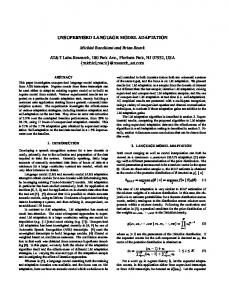
Show flights from Seattle
to Boston
ShowFlight ShowFlightCmd PreDCity City PostDCity PreACity City PostDCity Figure 2. Dynamic Programming Trellis showing the Viterbi interpretation as a solid path. Other paths with lower probability are not shown, yet they are also used in the EM algorithm.
At runtime we used the Viterbi path to find the most likely semantic labels. The Viterbi path for the input “Show flights from Seattle to Boston” is shown in Figure 2. A simple pruning mechanism was used such that at each column of the trellis, no transition would be made out of a node if its score is smaller than a threshold minus the maximum score in the same column.
>A