A Sensor Fusion Approach to Improve Joint Angle and Angular Rate. Signals in Articulated Robots. Daniel Kubus, Corrado Guarino Lo Bianco, and Friedrich M.
2012 IEEE/RSJ International Conference on Intelligent Robots and Systems October 7-12, 2012. Vilamoura, Algarve, Portugal
A Sensor Fusion Approach to Improve Joint Angle and Angular Rate Signals in Articulated Robots Daniel Kubus, Corrado Guarino Lo Bianco, and Friedrich M. Wahl Abstract— Rotary encoders and resolvers are by far the most common sensors to measure joint angles in articulated robots. Since various control approaches require angular rates as well, resolvers and encoders are also employed to derive angular rate signals. Due to the involved differentiation operation, however, quantization noise may be augmented significantly. Advanced filtering approaches can only partially overcome this drawback. Therefore, direct measurement of angular rates is desirable. Due to advancements in manufacturing technology and pushed by applications in entertainment devices, MEMS gyroscopes have become an attractive alternative for angular rate measurement. Unfortunately, they are affected by bias and other non-negligible disturbances, which may be a serious problem if consistent joint angle and angular rate measurements are required. The proposed approach fuses encoder and angular rate signals to mitigate their major drawbacks - bias and quantization errors - by exploiting their individual strong points. Bias in the angular rate signal is eliminated by analyzing the deviation between the integrated angular rate signal and the encoder signal. Quantization errors in the encoder signal are reduced by a so-called complementary filter which blends the integrated angular rate output with the encoder signal. Apart from a description of the approach and a theoretical analysis of its characteristics, experimental results demonstrating the effectiveness of the approach in closed-loop control of articulated robots are presented.
I. INTRODUCTION In articulated robots, rotary encoders are widely used to measure joint angles. Often, encoder signals are also employed to derive angular velocities and less commonly angular accelerations [1]. Various state-of-the-art robot control approaches rely on velocity (and acceleration) signals – hence providing consistent joint angle and angular rate signals is a key issue. When deriving angular rate signals based on encoder signals, a trade-off between required encoder resolution (quantization noise), signal bandwidth, and signal delay has to be incurred – regardless whether probabilistic filtering techniques, classic FIR/IIR filtering or predictive approaches are applied. In recent years, inexpensive MEMS gyroscopes with acceptable noise levels and dynamic ranges have become commercially available and so the costs for direct angular rate sensing have dropped considerably. In contrast to fiber optic gyroscopes, MEMS gyroscopes are affordable for most robotics applications. Therefore, these sensors have become an interesting alternative for angular rate sensing. Nevertheless, MEMS gyroscopes still have Daniel Kubus and Friedrich M. Wahl are with the Inst. f¨ur Robotik und Prozessinformatik, TU Braunschweig, Germany {d.kubus, f.wahl}@tu-bs.de. Corrado Guarino Lo Bianco is with the Dip. di Ing. dell’Informazione, Universita‘ degli Studi di Parma, Italy
978-1-4673-1736-8/12/S31.00 ©2012 IEEE
some issues. The most important drawbacks are bias, scale factor, and misalignment errors, which may severely affect performance. In contrast to the latter errors, which may be considered as constant, the bias is rather a slowly varying random process and can only be compensated on-line. In contrast to MEMS gyroscopes, encoder signals do not suffer from bias problems but are affected by quantization noise, which may cause problems with control approaches. As a hypothetical alternative, gyroscope signals could be integrated to obtain joint angle signals. Surprisingly – assuming commercially available gyro resolutions, standard rotary encoders and gears as employed by major industrial robot manufacturers – integrated angular rate signals often prove to be smoother than encoder signals but unfortunately the drift of the integrated signal renders this approach unfeasible. Yet, angular rate signals can in fact be exploited to obtain smooth joint angle signals whereas encoder signals can be utilized to eliminate the bias in angular rate sensor signals. This paper introduces a model-free bias and quantization error compensator (BQE2) employing FIR filtering techniques. The remainder of the paper is structured as follows. Section II reviews related work. In Section III, the concept of the BQE2 is presented in detail and in Section IV its characteristics are analyzed. Section V shows the effectiveness of the approach in closed-loop control of articulated robots and Section VI concludes the paper. II. RELATED WORK Estimating the state of motion of joints involving linear or rotary motion is generally a well-investigated problem. Commonly, linear/rotary encoders or resolvers are employed to obtain position signals. In [2] various approaches to real-time velocity estimation based on encoder signals are reviewed. Apart from approaches involving FIR/IIR filters with non-negligible delays, two major classes of methods are distinguished: predictive postfiltering and linear state observers. While predictive postfiltering techniques (e.g. [3]) require explicit differentiation of the position signal, state observers (e.g. [4]), such as the linear Kalman filter (e.g. [5]), perform differentiation implicitly employing a system model. Other approaches utilize techniques involving numerical integration instead of differentiation to avoid the noise amplification problem connected to differentiation, e.g. [6]. The aforementioned approaches rely on a high number of encoder increments per time-step to provide reliable velocity estimates. Therefore, the estimation performance clearly deteriorates if the resolution of the encoder is reduced or low velocities are considered. Lee et al. [7] explicitly focus
2736
on low-resolution encoders and low velocities respectively. To reduce encoder resolution requirements and improve the signal quality for low angular rates, direct angular rate sensing has become an affordable alternative. But compared to their expensive fiber optic counterparts, state-of-the-art MEMS gyroscopes show bias and hence drift rates that are orders of magnitudes higher. Therefore, their bias can significantly deteriorate system performance when angular rate signals are employed in control systems. Moreover, estimating joint angles based on angular rate measurements alone is hardly possible as the bias accumulates rapidly over time. This problem is usually tackled by combining gyroscopes with other sensors that are not affected by bias. As similar problems also arise in aircraft and spacecraft engineering, the respective literature, e.g. [8], provides valuable insights into this problem. Up to now, several approaches for linear and angular velocity estimation have been proposed which are based on fusing accelerometer and encoder signals. Zhu et al. have proposed different observer-based and frequency-weighting approaches to obtain velocity estimates from linear acceleration sensors and encoders, e.g. [9]. In [10] encoder and acceleration sensor signals are fused by a Kalman filter. An interesting alternative to the Kalman filter is the socalled complementary filter, which constitutes a model-free sensor fusion approach for signals from different sensor modalities. In its simplest form it adds a low-pass filtered signal originating from one sensor to a high-pass filtered signal from another sensor. Obviously, this filter only works as intended if the disturbances affecting the sensors can be separated in the frequency domain. In [11] the principle of complementary filtering is briefly reviewed and its interesting relation to the Kalman filter is discussed. Recently, ChangSiu et al. proposed an adaptive complementary filter for attitude estimation with gyroscopes and accelerometers [12]. In contrast to the above mentioned approaches, the sensor fusion approach for angular rate sensors and encoders presented in [13] is capable of reducing both angular rate sensor bias and encoder quantization noise. The approach has been termed bias and quantization error compensator(BQE). In this paper, an enhanced BQE approach is presented: The basic technique has been generalized from single-joint systems to arbitrary articulated robots; the computational complexity of the bias compensation step has been reduced considerably; the disturbance transfer characteristics have been improved; the processing scheme and the complementary filtering step have been restructured and generalized. Furthermore, experimental results demonstrating the effectiveness of the approach in closed-loop robot control are presented. In [13] the BQE was inaccurately termed drift and offset compensator. III. BIAS AND QUANTIZATION ERROR REDUCTION A. Concept Overview In an articulated robot, a single-axis gyroscope measuring the angular rate of link j (assuming joint j connects links j −
1 and j) not only measures the angular rate caused by joint j but also the contributions of the previous j − 1 joints if their axes of rotation are not orthogonal to the current rotation axis of joint j. Based on the robot geometry, the angular rate of link j caused by joints 1 . . . j − 1 may be calculated by propagating the contribution of each joint through the kinematic chain [14]. In the remainder of the paper four indexes for scalar variables are distinguished: In ab xcd the left superscript a denotes the frame in which x is expressed; the left subscript b denotes the joints that contribute to x (b∗ means that joints j = 1 . . . b contribute to x); the right superscript c indicates the employed sensor modality and the processing steps applied to x; the right subscript d denotes the timestep. For instance, jj α˙ kg designates the angular rate of joint j expressed w.r.t. frame j measured by a gyroscope at timestep k. If the meaning is unambiguous, indexes are omitted for simplicity. jj−1 R designates the rotation matrix that transforms quantities expressed w.r.t. frame j − 1 to frame j. j j∗ ω denotes the vector of angular velocities expressed w.r.t. frame j containing the contributions of joints 1 . . . j. Using this notation, jj∗ ω is given by Eq. (1). j j∗ ω
= jj−1 R
j−1 (j−1)∗ω
+ z jj α˙ g
(1)
The angular rate around the z axis of joint j caused by the preceding j − 1 joints is given by Eq. (2). [ ] j ˙ g = jj−1 R j−1 (2) (j−1)∗ω (j−1)∗ α z
The most striking disadvantage of calculating the angular rate of joint j according to this approach is the increase of the noise level. As the gyroscope signals of the preceding joints are propagated through the kinematic chain, the noise covariances of the gyroscopes sum up, which may render this approach unattractive. Moreover, geometric parameter inaccuracies will also propagate through the chain and link flexibilities may additionally deteriorate the results. Due to the low cost of MEMS gyroscopes and their small size, two gyroscopes per joint may be employed instead to obtain jj α˙ g . One gyro is mounted on link j − 1, the other one on link j. The trade-off between noise level and number of gyros has to be made individually depending on the system characteristics and signal requirements. Fig. 1 shows the proposed processing scheme for joint j. Two angular rates (j−1)∗ α˙ g and j∗ α˙ g serve as inputs. j∗ α˙ g is provided by a gyro mounted on link j while (j−1)∗ α˙ g is provided either by a gyro mounted on link j − 1 or computed according to Eqs. 1- 2. The difference of the angular rates yields the angular rate of joint j denoted by ˙ g . j αe designates the joint angle provided by the encoder. jα The bias compensator block computes a bias signal that is low-pass filtered to suppress undesirable disturbance transfer characteristics and added to the angular rate signal which yields the angular rate output. The angular rate output j ˙αgb is then integrated using the joint angle output of the previous gbo time-step j αk−1 . The resulting signal and the encoder output e α are fed into a complementary filter which passes lowj frequency portions of the encoder signal and high-frequency
2737
j
z-1
g g
(j-1)*
gb
j
j
t
gb
g
High-pass filter
j*
Bias Compensator Rotary Encoder
Complementary filter
j
gbo
Low-pass filter
e j
Fig. 1. Simplified scheme of the BQE. First, the bias of the angular rate signal is estimated and eliminated by the bias compensator. Subsequently, the resulting angular rate signal is integrated. In the final processing step, a so-called complementary filter eliminates any remaining low-frequency disturbances in the integrated signal by a high-pass/low-pass combination.
portions of the integrated angular rate signal thus eliminating any remaining drift in the joint angle output while at the same time reducing high-frequency quantization noise of the encoder. The following two subsections focus on the bias compensator and the complementary filter. B. Bias Reduction The bias compensation step compares the encoder signal with a sliding integral of the angular rate signal to derive a bias estimate which is then low-pass filtered and added to the original angular rate signal. Fig. 2 illustrates the bias
of this function yields an estimate for the bias, which is compensated by shifting the angular rate signal, as shown in Fig. 2 d). Although conceptually very simple, the method proves very effective in reducing the bias. In a previous version of the approach presented in [13], general linear and quadratic functions for fitting have been discussed. As the bias proves to vary very slowly, quadratic functions already tend to overfit the data. Therefore, linear functions have been employed in the experimental section in [13]. By processing the encoder data as depicted in Fig. 2, a linear function passing through the origin can be employed for fitting instead of a general linear function hence reducing the filter complexity significantly. The effects on the disturbance transfer functions are discussed in the following section. To compute the difference between the signals in Fig. 2 b), the encoder signal has to be zeroed at the current time-step k. Therefore, the current encoder sample αke is subtracted from ez the previous samples. αk−i for i = 1 . . . N is computed at each time-step. ez e αk−i = αk−i − αke (3) To obtain the sliding integral of the angular rate signal, the angular rate signal is integrated backwards. gz αk−i = −∆t
i ∑
g α˙ k−j
(4)
j=1
a)
g
b)
Now, the difference between the modified encoder signal ez αk−i and the sliding angular rate integral is computed.
gz
gez gz ez ∆αk−i = αk−i − αk−i ez
c)
is then fitted to a linear function passing through the gez dk−i = ˆbk ∆t(−i). The bias estimate is given origin, i.e., ∆α by solving the least-squares line-fitting problem, which can easily be cast into an LTI filter. By restricting the best-fit line to pass through the origin, the computation of the bias estimate ˆbk is simplified significantly (cf. [13]).
i=0
i=N gez
d)
(5)
gez ∆αk−i
gb
b
1 ∑ gez ∆αk−i (−i) S2 (N ) i=1 N
Fig. 2. Basic steps of the bias elimination procedure: a) angular rate signal; b) integrated angular rate signal and modified encoder signal; c) the difference between the latter signals and the best-line fit; d) the original and corrected angular rate signal.
compensation procedure. The angular rate signal depicted in Fig. 2 a) is integrated backwards as depicted by the dashed line in Fig. 2 b). The solid line depicts the encoder signal. Note that the encoder output at time step k has been subtracted to zero αez at time-step k. Due to the bias in the angular rate signal, the integral of the angular rate drifts. As gyro bias varies slowly over time [15] and can thus be approximated by a constant offset in the analysis time window, the drift of the integrated rate signal should closely resemble a linear function. To eliminate the bias, the difference αez − αgz , i.e., the dotted line in Fig. 2 c), is computed and a linear function passing through the origin is fitted – minimizing the least-squares error. The derivative
ˆbk =
(6)
After some manipulations one obtains the following equation: [ ] N ∑ 1 e e ˆbk = S1 (N )αk − αk−i i (7) ∆tS2 (N ) i=1 [N ] ∑ g 1 − α˙ (N + i)(N − i + 1) 2S2 (N ) i=1 k−i where S1 (N ) and S2 (N ) denote
2738
S1 (N ) =
N ∑ i=1
S2 (N ) =
N ∑ i=1
i2 =
1 N (N + 1) 2
(8)
1 (N + 3N 2 + 2N 3 ) 6
(9)
i=
To obtain the angular rate output α˙ gb , the current bias estimate is low-pass filtered and added to the current angular rate sensor output. The reasons for low-pass filtering and suitable filters are discussed in Section IV. α˙ gb = α˙ g + hlpb ∗ ˆbk
The central steps of the bias compensator are the computation of the bias estimate ˆbk and the subsequent addition of the low-pass filtered ˆbk to α˙ g . The Z transform of α˙ gb is given by 1 [αe (z)Ha (z) − α˙ g (z)Hb (z)] S2 (N ) (13) ] [ N ∑ 1 z −i (14) S1 (N ) − Ha (z) = ∆t i=1
(10)
α˙ gb (z) = α˙ g (z) +
C. Quantization Error Reduction To reduce encoder quantization errors, the proposed approach exploits the remarkable accuracy with which rotary motions can be measured by (inexpensive MEMS) gyroscopes within short time intervals. Owing to the integration of the angular rate signal (cf. Fig. 2), high-frequency noise of the gyroscope is well attenuated. Since the bias compensation step cannot completely remove the bias in α˙ g , the processed angular rate signal α˙ gb cannot simply be integrated to obtain the joint angle. Eq. 11 summarizes the integration step, in which the joint angle output of the previous time-step αgbo and the angular rate output of the bias elimination step α˙ kgb are added. gbo αkgb = αk−1 + α˙ kgb ∆t (11) To remove any drift in the integrated angular rate signal αgb , a complementary filter [11] is employed. The term complementary filter denotes a filter, whose transfer functions fulfill H2 (z) = 1 − H1 (z), as depicted in Fig. 3. In
H2 Basic complementary filter structure.
our case the encoder signal is low-pass filtered (impulse response hlpc ) to reduce encoder quantization noise while the angular rate integral is high-pass filtered (impulse response hhpc ) to prevent any drift in the resulting joint angle signal. The literature on complementary filtering and filter design in general is quite rich (e.g. [16]), so a detailed description is omitted. Since real-time control applications are targeted, low group delays of the employed filters are important. Although there exist better choices w.r.t. group delay, we have chosen a max-flat FIR design for simplicity here. The angular rate integral αkgb serves as one input for the complementary filter; the second input is the encoder signal αe . αkgbo = αgb ∗ hhpc + αe ∗ hlpc
i N i ∑ ∑ 1 ∑ −i i z −j = z (N +i)(N −i+1) (15) 2 i=1 i=1 j=1
Note that the low-pass filter has been omitted here to derive and analyze the pure disturbance transfer functions. The Z transform of the joint angle signal that is fed into the complementary filter is given by αgb (z) = α˙ gb (z)∆t + αgbo (z)z −1
(12)
αkgbo constitutes the joint angle output of the BQE2.
(17)
where HHP C (z) = 1 − HLP C (z). We employed a max-flat FIR filter design for the complementary filter although there are better choices w.r.t. the group delay. As can be inferred from the transfer functions, the BQE2 shows all-pass characteristics for both undisturbed angular rate and encoder signals. Since the BQE2 has two input signals that are affected by disturbances, four disturbance transfer functions (DTF) exist. To determine the disturbance transfer functions, α˙ g (z) and αe (z) in Eqs. 13-17 are replaced by the disturbance signals w(z) and v(z) respectively, i.e., α˙ g (z) = w(z) and αe (z) = v(z). The disturbance transfer characteristics of the joint angle output have already been analyzed in [13]. Owing to the changes in the bias estimation step and the optimization of the structure and the design of the complementary filter, these disturbance functions have been optimized further. A noteworthy issue with the initial approach BQE1 are the unfavorable disturbance characteristics of the angular rate output. Therefore, this paper focuses on the disturbance transfer functions Twα˙ and Tvα˙ . Twα˙ =
IV. ANALYSIS In the previous section the BQE2 has been described in the time domain. This section focuses on its characteristics in the Z domain. Since line fitting employing the least-squares error measure can be cast into an FIR filter as shown in the preceding section, the BQE2 can be analyzed using the theory of linear time-invariant (LTI) systems.
(16)
The complementary filter is basically a low-pass/high-pass combination in our case which passes high-frequency portions of αgb and low-frequency portions of αe thus eliminating any remaining drift in αgb and at the same time reducing the quantization error in the joint angle output. The transfer function of the complementary filter is given by αgbo (z) = HHP C (z)αgb (z) + HLP C (z)αe (z)
H1
Fig. 3.
Hb (z) =
α˙ gb (z) α˙ gb (z) Tvα˙ = w(z) v(z)
(18a-b)
The first index of the disturbance transfer function denotes the disturbance variable (w(z) or v(z)) and the second index denotes the output of the BQE (α˙ gb (z)). Figs. 4 and 5 show the magnitude of the frequency response of the DTFs Twα˙ and Tvα˙ of BQE1 [13] and BQE2 for different filter lengths N . Please note that the
2739
frequency axes are normalized such that ω = 2π corresponds to the sampling frequency Ωs . In contrast to the DTF Tvα˙ of BQE1, the corresponding DTF of BQE2 shows a lower maximum but oscillates at considerably higher values than Tvα˙ of BQE1. Thus, on first sight, BQE2 seems to have worse disturbance characteristics. However, the bias estimate ˆb is low-pass filtered before adding it to α˙ g . Hence, the transfer function Tvα˙ will not affect the angular rate output considerably if the low-pass filter (in our case a CIC filter based on [17]) is chosen properly. Regarding the DTF Twα˙ , an advantageous decrease of the maximum value and the initial slope can be observed for BQE2. All in all, BQE2 shows more favorable disturbance transfer characteristics than BQE1. For more details on the disturbance characteristics, esp. concerning the reduction of quantization errors, please consult [13].
Tw
N=25 N=50
b)
Fig. 5. DTFs showing the effects of disturbance in the angular rate signal α˙ g on the angular rate output α˙ gb for two different filter lengths. a) denotes the DTFs of BQE1 [13] while b) denotes the DTFs of BQE2, as presented in this paper. Both the slope and the maximum of the DTF have been reduced by the new approach. As can be seen, low-frequency disturbances - such as bias - are well attenuated.
placement of the IMUs and the parameters of the trajectories are depicted in Fig 6. The amplitude A and frequency f of T1 result in maximum joint velocities of α˙ ≈ 292◦ 1s , which is close to the maximum permissible joint velocity of the robot and the limits of the gyro. The maximum joint velocities of T2 and T3 are approx. α˙ ≈ 150◦ 1s , those of T4 α˙ ≈ 75◦ 1s .
N=25 N=50
Tv
a)
b)
T1 fj2 = 2.9Hz fj3 = 3.1Hz T2
a)
fj2 = 5.8Hz fj3 = 6.2Hz
Fig. 4. DTFs quantifying the effects of disturbance in the encoder signal αe on the angular rate output α˙ gb for two different filter lengths. a) denotes the DTFs of BQE1 [13] while b) denotes the DTFs of BQE2, as presented in this paper. The maximum of the DTFs are lower for the BQE2 bias estimation variant.
V. EXPERIMENTAL RESULTS In this section the effectiveness of the approach is demonstrated in the context of closed-loop robot control. For a detailed discussion of the performance of the original approach for joint angle and angular rate estimation (employing a precision encoder as ground truth source) we refer the reader to [13]. In this section, we restrict ourselves to closed loop control of robot manipulators to demonstrate the benefit for the control of articulated robots. Instead of a single-axis angular rate sensor, which would be sufficient, two MEMS IMUs (Analog Devices ADIS 16364) have been mounted on links 2 and 3 of a 6-DoF industrial manipulator but only one angular rate sensor per IMU has been used in the experiments. To assess the effectiveness of the approach, the following error of joints 2 and 3 is evaluated for four different sinusoidal trajectories. The
T3 fj2 = 0.7Hz fj3 = 0.75Hz T4 fj2 = 0.7Hz fj3 = 0.75Hz
Aj2 = 16.0◦ Aj3 = 15.0◦ Aj2 = 4.0◦ Aj3 = 3.75◦ Aj2 = 34.0◦ Aj3 = 32.0◦ Aj2 = 17.0◦ Aj3 = 16.0◦
Fig. 6. Left: Industrial robot St¨aubli RX 60 with inertial measurement units a and b attached to links 2 and 3. Right: Parameters of the test trajectories T1 and T2 .
The robot controller runs at 1kHz, features a position interface and employs a cascaded PID controller with velocity feedforward [18], whose output is fed to the frequency inverters. To evaluate the performance of BQE1 and BQE2 in closed-loop control, four signal configurations have been examined: 1) Joint angle provided by encoder; angular rate computed by numerical differentiation and low-pass filtering (max-flat FIR filter; group delay: 4 samples) of encoder output 2) Joint angle provided by encoder, angular rate provided by gyros 3) Joint angle and angular rate provided by BQE1 4) Joint angle and angular rate provided by BQE2 The trajectories for joints 2 and 3 have been executed for a period of approx 90s. To inject additional disturbance
2740
TABLE I
tweaking the involved filters – especially w.r.t. their group delay and cut-off frequencies – to further reduce the sensitivity of the outputs to quantization noise. Moreover, time-varying scale factor errors may be compensated by extending the presented approach accordingly. Apart from rotary motion, similar approaches may be applied to estimate positions, linear velocities, and linear accelerations by fusing linear acceleration sensors and linear encoders.
N ORMALIZED MEAN ABSOLUTE FOLLOWING ERROR FOR DIFFERENT SIGNAL CONFIGURATIONS
Trajectory and Joint T j j2 T1 j3 j2 T2 j3 j2 T3 j3 j2 T4 j3
1) 1 1 1 1 1 1 1 1
Configuration 2) 3) 0.923 0.887 0.944 0.891 0.904 0.865 0.931 0.874 0.873 0.838 0.889 0.849 0.861 0.831 0.865 0.834
4) 0.852 0.860 0.842 0.857 0.817 0.820 0.816 0.836
VII. ACKNOWLEDGMENTS We would like to thank the German Academic Exchange Service (DAAD) for supporting this work within the framework of the Vigoni programme.
orthogonal to the sensing direction of the gyroscopes, a sinusoidal trajectory (A1 = 10◦ and f1 = 2.0Hz) is applied to joint 1. The following error is measured by the mean absolute error (MAE) and normalized w.r.t. signal configuration 1). The results are summarized in Table I. In configuration 1) the numeric differentiation step increases the noise level – especially in low-velocity regions – which leads to the highest following error in the experiments. The employed low-pass filter does not cause a notable signal delay. Utilizing the unfiltered angular rate signals instead of the encoder-based angular rate signal (configuration 2)) yields a considerable decrease of the following error compared to configuration 1). If BQE1 or BQE2 is utilized to process the joint angle and angular rate signals, a further reduction of the following error can be achieved. BQE2 almost always outperforms BQE1. Especially, if trajectories with low joint velocities are executed, BQE is able to reduce the error significantly. Clearly, applying BQE1 or rather BQE2 is preferable to using the raw gyroscope and encoder signals. VI. CONCLUSION Robot control and parameter estimation approaches rely on precise and consistent joint angle and angular rate measurements. With the advent of inexpensive MEMS gyroscopes, direct angular rate sensing has become an affordable option for providing angular rate signals. The proposed approach fuses encoder signals with angular rate signals and exploits the main advantage of either sensor to compensate the major drawback of the other. Thus, both gyroscope bias and encoder quantization errors can be reduced. If angular rate signals are provided by inexpensive gyroscopes instead of deriving them from encoders, encoder resolution requirements may be relaxed considerably. Hence, overall system cost may be reduced while at the same time improving signal quality. Apart from single-joint systems and open loop applications – as addressed in [13] – the bias and quantization error compensator (BQE2) proves useful for closed-loop control of articulated robots, which has been demonstrated in the experimental section. Depending on the executed trajectory, the following error could be reduced by nearly 20%. The performance of the BQE2 may be improved further by
R EFERENCES [1] S. J. Ovaska and S. Valiviita. Angular acceleration measurement: A review. IEEE Transactions on Instrumentation and Measurement, 47(5):1211–1217, 1998. [2] R. J. E. Merry, M. J. G. van de Molengraft, and M. Steinbuch. Velocity and acceleration estimation for optical incremental encoders. Mechatronics, 20(1):709–718, 2010. [3] S. Valiviita and O. Vainio. Delayless differentiation algorithm and its efficient implementation for motion control applications. IEEE Transactions on Instrumentation and Measurement, 48(5):967–971, 1999. [4] K. Sakata and H. Fujimoto. Proposal of long sampling short cycle observer for quantization error reduction. In Proc. of the IEEE International Symposium on Industrial Electronics (ISIE), pages 1919– 1924, 2010. [5] P. R. B´elanger, P. Dobrovolny, A. Helmy, and X. Zhang. Estimation of angular velocity and acceleration from shaft-encoder measurements. The International Journal of Robotics Research, 17(11):1225–1233, 1998. [6] Y. X. Su, C. H. Zheng, P. C. Mueller, and B. Y. Duan. A simple improved velocity estimation for low-speed regions based on position measurements only. IEEE Transactions on Control Systems Technology, 14(5):937–942, 2006. [7] S. H. Lee, T. A. Lasky, and S. A. Velinsky. Improved velocity estimation for low-speed and transient regimes using low-resolution encoders. IEEE/ASME Transaction on Mechatronics, 9(3):553–560, 2004. [8] J. R. Wertz (Editor). Spacecraft Attitude Determination and Control. Springer, 1980. [9] W.-H. Zhu and T. Lamarche. Velocity estimation by using position and acceleration sensors. IEEE Transactions on Industrial Electronics, 54(5):2706–2715, 2007. [10] S. Jeon. State estimation based on kinematic models considering characteristics of sensors. In Proc. of the American Control Conference, pages 640–645, 2010. [11] W. T. Higgins Jr. A comparison of complementary and kalman filtering. IEEE Transactions on Aerospace and Electronic Systems, 11(3):321–325, 1975. [12] E. Chang-Siu, M. Tomizuka, and K. Kong. Time-varying complementary filtering for attitude estimation. In Proc. of International Conf. on Intelligent Robots and Systems, pages 2474–2480, 2011. [13] D. Kubus and F. M. Wahl. A sensor fusion approach to angle and angular rate estimation. In Proc. of IEEE International Conference on Intelligent Robots and Systems, pages 2481 – 2488, 2011. [14] K. Kozlowski. Modelling and Identification in Robotics. Advances in Industrial Control. Springer, 1998. [15] Z. Yinqiang, W. Shourong, and X. Dunzhu. Trend extraction of the mems gyroscope’s drift based on EEMD. In Proc. of the International Conference on Measuring Technology and Mechatronics Automation, volume 3, pages 1050–1053, 2010. [16] R. G. Lyons. Understanding Digital Signal Processing. Prentice Hall, 2011. [17] E. Hogenauer. An economical class of digital filters for decimation and interpolation. Acoustics, Speech and Signal Processing, IEEE Transactions on, 29(2):155 – 162, apr 1981. [18] A. Visioli. Practical PID Control. Springer, 2006.
2741