A search for outliers using the grand tour method is performed. ..... in blue. To answer this question we may use parallel-coordinate plot shown in Figure 2.
DSC 2001 Proceedings of the 2nd International Workshop on Distributed Statistical Computing March 15-17, Vienna, Austria http://www.ci.tuwien.ac.at/Conferences/DSC-2001 K. Hornik & F. Leisch (eds.) ISSN 1609-395X
A Set of XLispStat Subroutines for Detecting Outliers Anna Bartkowiak Institute of Computer Science, University of Wroclaw, PL
Abstract A search for outliers using the grand tour method is performed. The grand tour enables to inspect the configuration of the data points imagined as a data cloud located in multivariate space. In the proposed method we rotate the data cloud and inspect the projections in a scatterplot located in a 2D plane. The algorithm works in two windows. In the first one (exhibiting a plane) the projections of the rotated points onto a 2D plane are displayed. An ordinary or robust concentration ellipse with a given confidence level is superimposed in the same plane on the displayed points. Point-projections which fall outside the ellipse borders are suspected as outliers. In the second window a linked count plot is steadily recording how often the individual data points were notified outside the confidence borders. In such way we obtain suspected outliers (points falling frequently outside the borders of the confidence ellipse) and a clean data set constituted from points which were always notified as located inside the confidence ellipse. The procedure was tested using both benchmark data and some real data sets. The results of the tests were very satisfactory.
1
The need of a tool detecting and visualizing outliers
The aim of the paper is to present a set of XLispStat subroutines which may serve as a tool for detecting outliers and obtaining a clean subset. The problem of identifying outliers is since many years present in statistical data analysis – see the
Proceedings of DSC 2001
2
survey in a recent paper by Billor, Hadi and Velleman [8], see also other papers on that subject, e.g. Atkinson [2], Rocke and Woodruff [12], Rousseeuw and van Driessen [13]. Generally, the contemporary used algorithms are hybrid algorithms based on mathematical considerations and random restarts. They exploit the concept of Mahalanobis distance, which for an outlier is expected to appear big and significant. Let us recall that the Mahalanobis distance for a data point x = (x1 , x2 , . . . , xp ) from an assumed central point x0 = (x01 , x02 , . . . , x0p ) is defined as: D2 (x, x0 ) = (x − x0 )S−1 (x − x0 )T , with p denoting the number of variables, and S the covariance matrix evaluated from the data. Both x0 and S may be evaluated in a robust way. An outlier is a data point which somehow does not much the configuration exhibited by the majority of the analyzed data points – and sticks out in some directions. Thus an outlier should have a large Mahalanobis distance. When the distance is large? This is usually judged by establishing a kind of statistical significance, exploiting usually the assumption that – at least asymptotically – the Mahalanobis distances are distributed χ2p . This is certainly true for data having a multivariate normal distribution, but such distributions happen rarely in practice. The graphical procedure using the concept of the grand tour exploits the analyzed data set as it is, thus the assumption of normality is not so important.
2
The grand tour for detecting outliers
In this section we introduce firstly the idea of the grand tour. Next we show, how this method can be used for detecting outliers.
2.1
The idea of the grand tour
The idea of the grand tour is connected with D. Asimov who used that term in a paper in 1985 [1]. His idea was to obtain views of multivariate points through a series of projections, chosen to be dense in the set of all projections. As a result a sequence of two-dimensional scatterplots could be obtained which, asymptotically, would come arbitrarily close to all 2–dimensional scatterplots projectable from the given data. Asimov has outlined some methods which could serve to attain the goal, however the methods are presented rather in sketch, without giving the details. The idea of viewing a multivariate space by the grand tour was very attractive for data analysts. It was idependently implemented by Tierney in XLispStat [15] and by Swayne et. al. in XGobi [14]. Later Bartkowiak and Szustalewicz developed their own algorithm [3, 4] specifically with the aim to detect outliers. Huh et al. [11] have used the grand tour for tracking Korea census data consisting of 12 958 181 ordinary households with 31 variables (the presented in [11] analysis is based on 7 of them); generally: the proposed TGT (Tracked Grand Tour) enables the viewers the tracking of the touring process of each data point.
Proceedings of DSC 2001
2.2
3
Detecting outliers when running a grand tour
The grand tour enables to inspect the configuration of the data points located in multivariate space and imagined as a data cloud. One may say that the points are viewed from various directions. The outliers - containing atypical values either in the magnitude or in the structural relations between the variables – should stick out somehow from the data cloud, which should be observable when performing the rotations. In the proposed method we rotate the data cloud and inspect the projections in a 2D plane which exhibits a scatterplot of the projected points. Mathematically rotation means an orthogonal transformation. Bartkowiak and Szustalewicz [3, 4] have derived the formula for such a rotation based on random generation of two points on the hypersphere, in which the data cloud is enclosed. The proposed algorithm works in two windows. In the first one the projections of the rotated points onto a 2D plane are displayed. An ordinary or robust concentration ellipse with a given confidence level is superimposed in the same plane on the displayed points. Point-projections which fall outside the ellipse borders are suspected as outliers. In the second window a linked count plot is steadily recording how often the individual data points were notified outside the confidence borders. In such way we obtain suspected outliers (points falling frequently outside the borders of the confidence ellipse) and a clean data set constituted from points which were always notified as located inside the confidence ellipse. This method was investigated on many data sets – and it has worked fine. A thorough comparison of results obtained for some known benchmark data is in preparation [6]. An exemplary output for some liver disorders data is shown in Figure 1. Quite a crucial point of the algorithm is the way of constructing the concentration ellipses. We return to this point in next section.
3
Some details of implementation in XLispStat
In this section we present briefly our implementation of the grand tour with the special aim to detect outliers.
3.1
A survey of the subroutines
The method is implemented in several pieces of XLispStat code. For convenience, these pieces got the generic name of ‘subroutines’, although they contain rather ‘scripts’ or code of ’functions’. These scripts operate on a data set, which has the global name d-xx and is an array of p column arrays, each column array containing values for one (subsequent) variable. The following ‘subroutines’ are available: proc5 - initializes some constants, like number of directions, alpha, chi denoting the (1-alpha) quantile of the chi-square distribution with 2 degrees of freedom,
Proceedings of DSC 2001
4
and chi–sqrt – the square root of the derived quantile. The file proc5 provides also the functions: • std(x) and std-all(d-xx) standardizing for mean=0 and standard deviation=1 the n × 1 array x and the entire n × p data table d-xx, • mah2 – computing Mahalanobis distances for a bivariate variable (x, y) with n realizations, • ellk – computing and drawing an concentration ellipse, • sphere–rand – generating random point on hypersphere; ellkr - computing and drawing a robust concentration ellipse; ellk me - computing and drawing an ordinary concentration ellipse centered in the median center. Both ellkr and ellk me may be called at arbitrary time of the computing; if so, they overshade the actually active procedure (‘ellk’, ‘ellkr’, ‘ellk me’) for drawing the concentration ellipse; piece1 - creates two objects called mp3 (my-plot) and ip (index plot) – which are initialized as two graphical windows in the screen. The user may adjust them; piece2 – runs the proper grand tour. After generating a new direction a random number of rotations by a small angle is carried out; after each rotation the rotated points are projected onto mp3, next a new concentration ellipse is drawed and the count plot IP is adjusted for those points which were notified outside the concentration ellipse.
3.2
Ordinary or robust concentration ellipses
It is known that the outliers hidden in the data may inflate and distort the covariances evaluated from the data. This fact may have a doubly unfavorably effect: (1) data points which are truly outliers – because of the inflation – may not appear at an outstanding position e.g. in graphs exhibiting Q-Q plots of Mahalanobis distances or principal coordinates and (2) points which are ‘normal’, may appear there as outliers (due to the swamping effect). To avoid these effects, it is advisable to use concentration ellipses based on covariances estimated in a robust way. Methods for estimating robust covariances are well known [2, 12, 13, 8, 6], none the less they are mostly iterative and far too expensive for applying in our grand tour, where hundreds or thousands evaluations of concentration ellipses are needed. Seemingly cheap (from computational point of view) is a procedure described in an early paper by Gnanadesikan and Kettenring [10] and called by us in the following the DSD method. It starts from the identity that a covariance of X, Y may be computed as the difference between the variances of U 1 = X + Y and U2 = X − Y : cov(X, Y ) = 0.25[var(X + Y ) − var(X − Y )] = 0.25[var(U 1) − var(U 2)].
(1)
Proceedings of DSC 2001
5
The gain from such a more complicated calculations by formula (1) is that the variances var(U 1) and var(U 2) may be now estimated by a robust method, using e.g., the MAD statistics, i.e. the Median of Absolute Deviations from the median: d ) = M AD(U )/0.675. var(U The computations by the just introduced DSD method are relatively cheap, however the covariance matrices with elements evaluated by that method are nor necessarily positive-definite (p.d.), in fact, they may be even negative-definite (n.d.). One may approximate such a n.d. matrix by the nearest (p.d.) matrix in Rp×p [9, 7]. The method needs further testing. Meanwhile let us notice the following: In the grand tour we do not construct truly multivariate covariance matrices for observed variables; we construct the concentration ellipses only from two derived variables which are linear combinations of the original variables. Applying this robust estimation procedure to many real data sets and evaluating for each of them the robust concentration ellipse truly for hundreds time we have only occasionally (in single cases) noticed, that the procedure based on formula (1) has failed.
3.3
Why XLispStat?
We have implemented our set of subroutines for detecting outliers in XLispStat first of all because of the nice interactive graphics available in that system. the code of subroutines is short and efficient. One does not need to declare types of variables – they are recognized by the system. It works as an interpreter, the code of the functions is in ASCII and may be read and adjusted by any text editor. The graphical objects can be easily changed. Points may by selected and change their shape and color. Sets of selected points may be hidden or left in the window (with the un-selected hidden) for further analysis. And last but not least: XlispStat is freely accessible through the internet.
4
Examples of application
A comparative review of 7 methods of identifying outliers applied to 7 benchmark data sets is given in [6]. Further detailed analysis of the famous milk container data is presented in [5]. Here we illustrate the use of the grand tour for another data set: the Liver disorders, taken from the Irvine data repository 1 . The data were recorded in the BUPA Research Ltd. company and contain evaluations for patients complaining for liver disorders. ¿From these data we have taken records containing 5 blood tests which are thought to be sensitive to liver disorders that might arise from excessive alcohol consumption. Each record contains data for one male patients. The following 5 measurements (variables) were taken into consideration: 1
URL http://www.ics.uci.edu/pub/machine-learning-databases/
Proceedings of DSC 2001
6
1. mcv mean corpuscular volume 2. alkphos alkaline phosphotase 3. sgpt alamine aminotransferase 4. sgot aspartate aminotransferase 5. gammagt gamma–glutamyl transpeptidase For our analysis we have taken only a part of the data, namely n = 117 male patients which have declared that they do not take in principle alcoholic drinks (the number of half-pint equivalents of alcoholic beverages drunk per day has been declared as 0 or 0.5).
Figure 1: Two snapshots of the screen when running the grand tour for the liver disorders data. Left: Scatterplots containing the projected points with a robust 99% concentration ellipse evaluated by the DSD algorithm. Right: Corresponding count plots. The points no. 35, 52, 78, 97, 106 are selected as appearing frequently outside the borders of the concentration ellipse After a preliminary run of the grand tour with ordinary concentration ellipses we have decided to apply robust concentration ellipses with the confidence level β = 0.01. Two snapshots from the run are shown in Figure 1. One can see there that points no. 35, 52, 78, 97 and 106 were indicated as appearing most frequently outside the borders of the ellipse. Of course, when rotating the data cloud, in some
Proceedings of DSC 2001
7
projections the indicated points may appear outside, and in some projections inside the ellipse. E.g. the upper left plot indicates for the points 105, 35 and 97 as keeping outstanding positions; in another projection, shown in the bottom left plot these are points no. 35, 106, 52, 24 and 78, while the point 97 sticks closely to the main cloud of the data. The count plots indicate clearly that these 6 points are much suspected to be outliers. From the count plot we could also obtain a clean data set (‘clean’ means without outliers): constituted from points which have never appeared outside the borders of the concentration ellipse. Now another crucial question: Why the indicated points are suspected as outliers? What is special in these points?
Figure 2: Parallel coordinate plot exhibiting the liver disorders data. The segments for data points no. 35, 52, 78, 97, 106 – indicated by the grand tour as possible outliers are colored in red; segments for point no. 24, a minor outlier, are colored in blue To answer this question we may use parallel-coordinate plot shown in Figure 2. The code for this function may be found in the book by Tierney [15]. In Figure 2 each point is represented by a segment line connecting (unvisible) vertical axes standing for coordinate axes of the considered variables v1, v2, v3, v4, v5 (represented from left to right in the plot). One may see in Figure 2 that really the indicated points are outstanding; in particular the points 35 and 106 are quite different from the remaining ones.
References [1] D. Asimov. The grand tour. a tool for viewing multidimensional data. SIAM J. Sci. Stat. Comput., 6:128–143, 1985.
Proceedings of DSC 2001
8
[2] A.C. Atkinson. Fast very robust methods for the detection of multiple outliers. JASA, 89:1329–1339, 1994. [3] A. Bartkowiak and A. Szustalewicz. Detecting multivariate outliers by a grand tour. Machine Graphics & Vision, 6(4):487–505, 1997. [4] A. Bartkowiak and A. Szustalewicz. Watching steps of a grand tour implementation. Machine Graphics & Vision, 7:655–680, 1998. [5] A. Bartkowiak and A. Szustalewicz. Outliers – finding and classifying which genuine and which spurious. Computational Statistics, 15:3–12, 2000. [6] A. Bartkowiak and J. Zdziarek. Identifying outliers – a comparative review of 7 methods applied to 7 benchmark data sets. Manuscript pp. 1–16, 2001. [7] A. Bartkowiak and K. Zi¸etak. Correcting possible non–positiveness of a covariance matrix estimated elementwise in a robust way. In Advanced Computer Systems, ACS’2000, Proceedings, Szczecin – Poland – 23–25 October, pages 91–96, 2000. [8] N. Billor, A.S. Hadi, and P.F. Velleman. Bacon: blocked adaptive computationally efficient outlier nominators. Computational Statistics & Data Analysis, 34(3):279–298, 2000. [9] S.H. Cheng and N.J. Higham. A modified cholesky algorithm based on symmetric indefinite factorization. SIAM J. Matrix Anal. Appl., 19:1097–1110, 1998. [10] R. Gnanadesikan and J.R. Kettenring. Robust estimates, residuals and outlier detection. Biometrics, 28:81–124, 1972. [11] M.Y. Huh, Jang Oe.K., Kim K.Y., and Song K.R. Statistical information visualization on the network. In Bulletin of the Intern. Statistical Institute (ISI99 52nd Session Proceedings, Invited papers) LVIII, 2, pages 111–114, 1999. [12] D.M. Rocke and D.L. Woodruff. Identification of outliers in multivariate data. JASA, 91(435):1047–1061, 1996. [13] P.J. Rousseeuw and K. van Driessen. A fast algorithm for the minimum covariance determinant estimator. Technometrics, 41:212–223, 1999. [14] D.F. Swayne, D. Cook, and A. Buja. X-gobi, interactive dynamic graphics in the xwindows system with a link to s. In ASA Proc. Sect. on Statistical Graphics, pages 1–8, 1994. [15] L. Tierney. Lisp–Stat, an Object–Oriented Environment for Statistical Computing and Dynamic Graphics. Wiley, New York, 1990.