A Shape Constrained Curve Approximation Method for Styling Surfaces Modeling Yves Mineur University of Valenciennes CNRS, UMR 8530 LAMIH France BP311 59313 Valenciennes Cedex9
[email protected] ABSTRACT The problem of styling surfaces modeling is tackled. An approach based on section curves fairing is chosen. The concept of template curves is developed for approximating profiles with a monotone curvature variation. Constrained Bezier curves called typical curves are used for that. A curve growing process based on a G2 typical curve fitting method, is investigated. It consists first in determining a seed curve element then by a succession of extrapolating and fitting operations, to generate a curve segment with a given monotone curvature variation fitted locally to a data points set.
Keywords Styling surfaces, Curve fairing, Monotone curvature, Shape preservation.
1. INTRODUCTION The styling surfaces are encountered in an increasing number of products, the most representative ones being the car bodies. Their main characteristics are linked to their aesthetical expected role. The experience shows that the aesthetic of such shapes is closely linked to their curvature profile. A monotone and convex curvature variation is generally expected [Buc92]. Achieving these characteristics by using the classical geometrical modeling or approximating method is not easy when processing large raw data points sets. A major difficulty comes from the lack of these methods to operate an efficient shape discrimination or smoothing without losing some details on the curvature variation. So, in the practice, it is often required, and some times preferred too, to adjust the shape manually, by directly moving the control points, to get the desired results. However, modeling fair surfaces in this way remains a tedious work and requires a good Permission to make digital or hard copies of all or part of this work for personal or classroom use is granted without fee provided that copies are not made or distributed for profit or commercial advantage and that copies bear this notice and the full citation on the first page. To copy otherwise, or republish, to post on servers or to redistribute to lists, requires prior specific permission and/or a fee. WSCG POSTERS proceedings WSCG’2003, February 3-7, 2003, Plzen, Czech Republic. Copyright UNION Agency – Science Press
experience. A usual approach to handle this problem consists in fairing first a set of sections, then to generate surfaces between these sections by using blending or interpolation functions. Starting from this methodology, our work aims to develop a curve approximating method integrating design specifications of styling surfaces. We considered more precisely the problem of approximating a data points set by a composite G2 Bezier curve with a smooth varying curvature. This paper presents the first steps of this development and the main related concepts.
2. THE TEMPLATE CURVES MODELING APPROACH The approach we had is quite similar to the process used in the past to draw manually the car bodies section lines (figure 1). It worked by using template or pre-defined curves with a given curvature profile. A draw thereby was the result of adjacent given shaped curves selected according a shape matching principle. Numerous shape constrained or preserved modeling methods have been considered for such a purpose. Relevant issues concerning the generation of fair visually pleasant or aesthetical- shapes can be found in [Hig88],[Miu00]. They are however not suited to the curve approximation. In a previous work, [Min98], an element of solution to this problem has been provided.
Form 1
Translation 2
Until Curve Generation Completion Set of Template Curves
Fitting 3
partly verifies the properties of the pythagoreanhodograph (PH) curves [Far90] whose interest for generating fair curves have been confirmed [Alb96] [Wal96] . Cubic typical curves seem to be suited to our problem. However, for a more suitable use, we define a new parameters set, called the form parameters. They consist in the curvature κ0 at the end point C(u=0), the curve arc length ∆S and the angle between the end tangents ∆W The relations between the form and canonical parameters are :
Figure 1 : Section drawing by using template curves
∆W = 2ϕ
(3)
∆S = l (1+ hcosϕ + h )
(4)
3∆Sκ0 = 2h sinϕ + h sin2ϕ + 2h sin ϕ
(5)
2
3
3.THE TYPICAL CURVES TEMPLATE CURVES.
AS
The notion of typical curves, defined in [Min98], derives from a Bezier curve definition proposed in [Hig88]. A typical curve is a curve whose definition is partially constrained in order to provide a monotone curvature variation. The definition parameters of a typical curve, we will call them the canonical parameters, are (figure 2) : - l for the length of the first control polygon edge, - h and ϕ respectively for the length ratio and the angle between control polygon edges.
ϕ
hl
ϕ
h2l
l
ϕ h3l
Figure 2 : 4th Degree Typical Curve The typical curves have many interesting properties. Their arc length differential and their curvature can be directly evaluate from the following expressions of the curve definition parameter:
ds (u)=mla du
κ (u )= m −1 m
with
m−1 2
hsinϕ 1 m +1 l a 2
2
(1) (2)
a = 1+2(hcosϕ -1)u+(1-2 h cosϕ + h2)u2 and where m is the curve degree. In the case of 3rd degree typical curves, the arc length differential becomes a polynomial and thus
4. STATEMENT OF THE PROBLEM. The problem that we considered, can be expressed in these terms: Given a data points set, find a composite (segmented) G2 Bezier curve which is fitted to data points and with a smooth and monotone varying curvature. A major sub-problem inherent to such an approximation is to locate a part of a the data points set compatible with a single typical curve shape and offering good continuity conditions with the adjacent curves. Same reasoning are encountered in the segmentation methods by region growing [Sap95]. Our orientation was to transpose this previous method to our problem. A particularity in our case lies in the requirement of G2 continuity conditions. The curve growing process that we intend to develop suppose at the beginning the choice of a starting point and of a growing direction. Starting point (G2 continuity Growing direction conditions) 1 : Curve extrapolation 2 : Curve fitting Data points
#i growing step #i+1 growing step
Figure 3 : Multi-steps extrapolation-fitting or growing curve process Without considering more in details this choice, it leads to consider the elementary problem of extrapolating a cubic typical curve and fitting it
while satisfying a G2 continuity with a previous curve segment (figure 3). For the sake of concision, we will not discuss in this paper of the extrapolation problem.
5. TYPICAL CURVE FITTING WITH G2 CONTINUITY CONDITIONS. We suppose the arc length of the typical curve to be fitted as fixed. Initial Curve (C) :∆S, ∆W C(1) Initial conditions P0 , W0, κ0
dC dϕ
P1 Data Points Polygonal Line (DP)
∂F ∂l ∂F + ∂l ∂ϕ ∂h ∂G ∂l ∂G + ∂l ∂ϕ ∂h
∂h ∂F + = 0 ∂ϕ ∂ϕ ∂h ∂G + = 0 ∂ϕ ∂ϕ
(8)
which unknowns are the partial derivatives of l and h with respect to ϕ. From their calculation, the previous displacement gradient vector of the end point C(1), is thus determined. The fitting procedure then leads to determine on the data polygonal line DP , the point P1 at the intersection with the displacement gradient vector (figure 4), then by making ∆C = C(1)P in the relation (6), to 1
Figure 4 : Cubic typical curve fitting procedure Let DP the polygonal line to be approximated, and C(u) for u ∈[0,1], the cubic typical curve to be fitted. The considered continuity conditions are the point position P0 at the curve end point C(0), the tangent direction W0 and the curvature κ0 at this point. Considering the form parameters definition (see section 3), the fitting process is then to find a proper value for ∆W so that the curve becomes as close as possible to the data points. The approach is thus the following. Let (Oxy) be a local frame defined from the point P0 and the vector W0 taken as the x axis direction. We define first an initial curve satisfying the initial conditions with an arbitrary value for ∆W. We will make the assumption that this initial curve is relatively close to the data points. Considering a given curve point C(u), its displacement ∆C when modifying ∆W by a variation δW can be expressed by approximation as :
1 dC ∆C = δW 2 dϕ
(6)
A convenient curve point where calculating the derivative d C is C(1). It comes thereby, relatively dϕ the frame (Oxy) and in a complex formalism, the expression :
π
jϕ + ∂l dC ∂ + ( u = 1) = ( hl )e jϕ + hle 2 ∂ϕ ∂ϕ dϕ
Considering furthermore the relations (4) and (5) as two implicit functions, denoted respectively F and G, of the parameters h, l, ϕ, we obtain by differentiation the following equations system :
π
j 2ϕ + ∂ 2 + ( h 2 l )e j 2ϕ + 2h 2 le ∂ϕ
(7)
calculate the corresponding variation δW on ∆W.
6. CURVE APPROXIMATION METHOD OVERVIEW AND EXPERIMENTATION . Our method consists in three main steps: 1 :A seed element or curve is calculated. Such a curve is supposed to be small and fitted to the data points. 2 :The previous curve segment is extrapolated and fitted to the data points. 3 : The fitting quality is assessed. The step 2 is iterated while the fitting quality (step 3) is considered as achieved. As soon as the fitting goodness requirements cannot be achieved, the growing process is stopped and a new curve segment is processed according to the whole previous steps. An illustrating example The figure 5 shows two successive curve growing steps. The considered curve is connected to a first fitted typical curve. We will note here that the obtained curvature variation is particularly fair. The advantage of the typical curves is to ensure by their intrinsic form characteristics a natural noise filtering. Assessment of the fitting goodness Concerning the fitting accuracy, a classical curve deviation diagnosis, by measuring the distances between the curve and the data points, proved here to be not reliable to stop a curve growing. The problem is to set properly the curve segmentation so that the curvature variation on the approximation curve matches the one underlying to the data points.
1st arc 2nd arc after extrapolation
G2 continuity
Data points
after fitting
Figure 5 : Cubic typical curve growing The solution that we implemented, consists in evaluating, at each growing step, a normal vector from the data points lying in neighborhood of the fitted curve end point. When the normal vector on the fitted curve deviates from the estimated local normal vector of a given threshold value, the growing process is stopped. A difficulty obviously is to set properly the maximal allowed deviation.
useful materials for direct applications in styling surfaces modeling. The curvature variation profile inherent to the typical curve definition can be seen as an ideal one for styling shapes modeling. The different tests performed on various data points sets have shown that these curves are well suited to the shape approximation in automotive design. The new composite typical curve fitting method we investigate nevertheless fails to work properly in some cases. The main encountered problem concerns the shape recognition. Our future work will deal with the integration in our curve growing process of a data points pre-processing phase. The aim is to get a global curvature variation estimation in order to control and to weight in a fitted way the different process parameters such as the extrapolation rate or the curve fitting displacement vector.
8. ACKNOWLEDGMENTS The author would like to thank the ICEM Technologies GmbH company in Hannover (Germany) where this research was carried out.
Semi-automatic processing
9. REFERENCES
Because of the previous problem, it can nevertheless happen that the growing process stops on a inappropriate location. However our method can be used in a semi-automatic mode by setting in advance the segmentation points as shown in figure 6. The problem of G2 bi-arcs fitting, frequently met in styling surfaces modeling, thus could be solved in a safer way than with a classical least-squares approximation. Manually set 1st arc segmentation points
[Alb96] G.Albrecht, R.T.Farouki : Construction of C2 Pythagorean-hodograph interpolating splines by the homotopy method. Advances in computational Mathematics 5(1996)PP417-442
2nd arc Typical curves fitting
[Buc92] Buchard, H.G.Ayers, J.A.Frey, Sapidis Approximation with aesthetic constraints .. GM Res. Publ. SIAM 1992 [Far90] R.T.Farouki, T.Sakkalis. Phytagorean Hodographs. IBM J.Res. Develpo. 34 (1990) pp736752 [Hig88] M.Higashi, K.Kaneko Generation of HighQuality Curve and Surface with Smoothly Varying Curvature.. Eurographics’88. PP79-93. [Min98] Y.Mineur, T.Lichah, JM.Castelain, H.Giaume. A shape controlled Fitting Method for Bezier Curves. CAGD (1998) V.15 pp 879-881
Expected maximum curvature point Least squares fitting Figure 6 : Bi-arcs fitting on a rounded corner shape
7. CONCLUSIONS AND PROSPECTS The work presented in this report cannot be considered as finished. It results from this however,
[Miu00] . K.T.Miura. Unit Quaternion integral curve : A new type of fair free-form curves. CAGD (2000) V.17 pp39-58 [Sap95] N.S.Sapidis, P.J.Besl. Direct construction of polynomial surfaces from dense range images through region growing.. ACM Transactions on Graphics (1995) V.14 pp171-200 [Wal96] D.J.Walton, D.S.Meek. A Pythagorean hodograph quintic spiral.. CAD (1996) V.28 pp943950.