A Short Introduction to Model Selection, Kolmogorov Complexity and

A Short Introduction to Model Selection, Kolmogorov Complexity and Minimum Description Length (MDL)∗

arXiv:1005.2364v2 [cs.LG] 14 May 2010

Volker Nannen

Abstract The concept of overfitting in model selection is explained and demonstrated. After providing some background information on information theory and Kolmogorov complexity, we provide a short explanation of Minimum Description Length and error minimization. We conclude with a discussion of the typical features of overfitting in model selection.

1

The paradox of overfitting

Machine learning is the branch of Artificial Intelligence that deals with learning algorithms. Learning is a figurative description of what in ordinary science is also known as model selection and generalization. In computer science a model is a set of binary encoded values or strings, often the parameters of a function or statistical distribution. Models that parameterize the same function or distribution are called a family. Models of the same family are usually indexed by the number of parameters involved. This number of parameters is also called the degree or the dimension of the model. To learn some real world phenomenon means to take some examples of the phenomenon and to select a model that describes them well. When such a model can also be used to describe instances of the same phenomenon that it was not trained on we say that it generalizes well or that it has a small generalization error. The task of a learning algorithm is to minimize this generalization error. Classical learning algorithms did not allow for logical dependencies [MP69] and were not very interesting to Artificial Intelligence. The advance of techniques like neural networks with back-propagation in the 1980’s and Bayesian networks in the 1990’s has changed this profoundly. With such techniques it is possible to learn very complex relations. Learning algorithms are now extensively used in applications like expert systems, computer vision and language recognition. Machine learning has earned itself a central position in Artificial Intelligence. A serious problem of most of the common learning algorithms is overfitting. Overfitting occurs when the models describe the examples better and better ∗ The

Paradox of Overfitting [Nan03], Chapter 1.

2

AN EXAMPLE OF OVERFITTING

but get worse and worse on other instances of the same phenomenon. This can make the whole learning process worthless. A good way to observe overfitting is to split a number of examples in two, a training set, and a test set and to train the models on the training set. Clearly, the higher the degree of the model, the more information the model will contain about the training set. But when we look at the generalization error of the models on the test set, we will usually see that after an initial phase of improvement the generalization error suddenly becomes catastrophically bad. To the uninitiated student this takes some effort to accept since it apparently contradicts the basic empirical truth that more information will not lead to worse predictions. We may well call this the paradox of overfitting. It might seem at first that overfitting is a problem specific to machine learning with its use of very complex models. And as some model families suffer less from overfitting than others the ultimate answer might be a model family that is entirely free from overfitting. But overfitting is a very general problem that has been known to statistics for a long time. And as overfitting is not the only constraint on models it will not be solved by searching for model families that are entirely free of it. Many families of models are essential to their field because of speed, accuracy, easy to teach mathematically, and other properties that are unlikely to be matched by an equivalent family that is free from overfitting. As an example, polynomials are used widely throughout all of science because of their many algorithmic advantages. They suffer very badly from overfitting. ARMA models are essential to signal processing and are often used to model time series. They also suffer badly from overfitting. If we want to use the model with the best algorithmic properties for our application we need a theory that can select the best model from any arbitrary family.

2

An example of overfitting

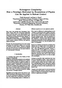
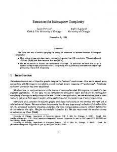
Figure 1 on page 3 gives a good example of overfitting. The upper graph shows two curves in the two-dimensional plane. One of the curves is a segment of the Lorenz attractor, the other a 43-degree polynomial. A Lorenz attractor is a complicated self similar object. Here it is only important because it is definitely not a polynomial and because its curve is relatively smooth. Such a curve can be approximated well by a polynomial. An n-degree polynomial is a function of the form f (x) = a0 + a1 x + a2 x2 + · · · + an xn ,

x∈R

(1)

with an n + 1-dimensional parameter space (a0 . . . an ) ∈ Rn+1 . A polynomial is very easy to work with and polynomials are used throughout science to model (or approximate) other functions. If the other function has to be inferred from a sample of points that witness that function, the problem is called a regression problem. Based on a small training sample that witnesses our Lorenz attractor we search for a polynomial that optimally predicts future points that follow the same 2

2

AN EXAMPLE OF OVERFITTING

Figure 1: An example of overfitting

Lorenz attractor and the optimum 43-degree polynomial (the curve with smaller oscillations). The points are the 300 point training sample and the 3,000 point test sample. Both samples are independently identically distributed. The distribution over the x-axis is uniform over the support interval [0, 10]. Along the y-axis, the deviation from the Lorenz attractor is Gaussian with variance σ 2 = 1.

Generalization (mean squared error on the test set) analysis for polynomials of degree 0–60. The x-axis shows the degree of the polynomial. The y-axis shows the generalization error on the test sample. It has logarithmic scale. The first value on the left is the 0-degree polynomial. It has a mean squared error of σ 2 = 18 on the test sample. To the right of it the generalization error slowly decreases until it reaches a global minimum of σ 2 = 2.7 at 43 degrees. After this the error shows a number of steep inclines and declines with local maxima that soon are much worse than the initial σ 2 = 18.

3

3

THE DEFINITION OF A GOOD MODEL

distribution as the training sample—they witness the same Lorenz attractor, the same noise along the y-axis and the same distribution over the x-axis. Such a sample is called i.i.d., independently identically distributed. Here the i.i.d. assumption will be the only assumption about training samples and samples that have to be predicted. The Lorenz attractor in the graph is witnessed by 3,300 points. To simulate the noise that is almost always polluting our measurements, the points deviate from the curve of the attractor by a small distance along the y-axis. They are uniformly distributed over the interval [0, 10] of the x-axis and are randomly divided into a 300 point training set and a 3,000 point test set. The interval [0, 10] of the x-axis is called the support. The generalization analysis in the lower graph of Figure 1 shows what happens if we approximate the 300 point training set by polynomials of rising degree and measure the generalization error of these polynomials on the 3,000 point test set. Of course, the more parameters we choose, the better the polynomial will approximate the training set until it eventually goes through every single point of the training set. This is not shown in the graph. What is shown is the generalization error on the 3,000 points of the i.i.d. test set. The x-axis shows the degrees of the polynomial and the y-axis shows the generalization error. Starting on the left with a 0-degree polynomial (which is nothing but the mean of the training set) we see that a polynomial that approximates the training set well will also approximate the test set. Slowly but surely, the more parameters the polynomial uses the smaller the generalization error becomes. In the center of the graph, at 43 degrees, the generalization error becomes almost zero. But then something unexpected happens, at least in the eyes of the uninitiated student. For polynomials of 44 degrees and higher the error on the test set rises very fast and soon becomes much bigger than the generalization error of even the 0-degree polynomial. Though these high degree polynomials continue to improve on the training set, they definitely do not approximate our Lorenz attractor any more. They overfit.

3

The definition of a good model

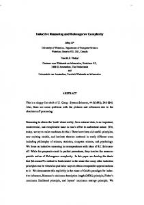
Before we can proceed with a more detailed analysis of model selection we need to answer one important question: what exactly is a good model. And one popular belief which is persistent even among professional statisticians has to be dismissed right from the beginning: the model that will achieve the lowest generalization error does not have to have the same degree or even be of the same family as the model that originally produced the data. To drive this idea home we use a simple 4-degree polynomial as a source function. This polynomial is witnessed by a 100 point training sample and a 3,000 point test sample. To simulate noise, the points are polluted by a Gaussian distribution of variance σ 2 = 1 along the y-axis. Along the x-axis they are uniformly distributed over the support interval [0, 10]. The graph of this example and the analysis of the generalization error are shown in Figure 2. The

4

3

THE DEFINITION OF A GOOD MODEL

generalization error shows that a 4-degree polynomial has a comparatively high generalization error. When trained on a sample of this size and noise there is only a very low probability that a 4-degree polynomial will ever show a satisfactory generalization error. Depending on the actual training sample the lowest generalization error is achieved for polynomials from 6 to 8 degrees. This discrepancy is not biased by inaccurate algorithms. Neither can it be dismissed as the result of an unfortunate selection of sample size, noise and model family. The same phenomenon can be witnessed for ARMA models and many others under many different circumstances but especially for small sample sizes. In [Rue89] a number of striking examples are given of rather innocent functions the output of which cannot reasonably be approximated by any function of the same family. Usually this happens when the output is very sensitive to minimal changes in the parameters. Still, the attractor of such a function can often be parameterized surprisingly well by a very different family of functions1 . For most practical purposes a good model is a model that minimizes the generalization error on future output of the process in question. But in the absence of further output even this is a weak definition. We might want to filter useful information from noise or to compress an overly redundant file into a more convenient format, as is often the case in video and audio applications. In this case we need to select a model for which the data is most typical in the sense that the data is a truly random member of the model and virtually indistinguishable from all its other members, except for the noise. It implies that all information that has been lost during filtering or lossy compression was noise of a truly random nature. This definition of a good model is entirely independent from a source and is known as minimum randomness deficiency. It will be discussed in more detail on page 12. We now have three definitions of a good model : 1. identifying family and degree of the original model for reconstruction purposes 2. minimum generalization error for data prediction 3. randomness deficiency for filters and lossy compression We have already seen that a model of the same family and degree as the original model does not necessarily minimize the generalization error.

The important question is: can the randomness deficiency and the generalization error be minimized by the same model selection method?

1

To add to the confusion, a function that accurately describes an attractor is often advocated as the original function. This can be compared to confusing a fingerprint with a DNA string. Both are unique identifiers of their bearer but only one contains his blueprint.

5

3

THE DEFINITION OF A GOOD MODEL

Figure 2: Defining a good model

Original 4-degree polynomial (green), 100 point training sample, 3,000 point test sample and 8-degree polynomial trained on the training sample (blue). In case you are reading a black and white print: the 8-degree polynomial lies above the 4-degree polynomial at the left peak and the middle valley and below the 4-degree polynomial at the right peak.

The analysis of the generalization error σ 2 . A 0-degree polynomial achieves σ 2 = 14 and a 4-degree polynomial σ 2 = 3.4 on the test sample. All polynomials in the range 6–18 degrees achieve σ 2 < 1.3 with a global minimum of σ 2 = 1.04 at 8 degrees. From 18 degrees onwards we witness overfitting. Different training samples of the same size might witness global minima for polynomials ranging from 6 to 8 degrees and overfitting may start from 10 degrees onwards. 4 degrees are always far worse than 6 degrees. The y-axis has logarithmic scale.

6

4

INFORMATION & COMPLEXITY THEORY

Such a general purpose method would simplify teaching and would enable many more people to deal with the problems of model selection. A general purpose method would also be very attractive to the embedded systems industry. Embedded systems often hardwire algorithms and cannot adapt them to specific needs. They have to be very economic with time, space and energy consumption. An algorithm that can effectively filter, compress and predict future data all at the same time would indeed be very useful. But before this question can be answered we have to introduce some mathematical theory.

4

Information & complexity theory

This section provides a raw overview of the essential concepts. The interested reader is referred to the literature, especially the textbooks Elements of Information Theory by Thomas M. Cover and Joy A. Thomas, [CT91] Introduction to Kolmogorov Complexity and Its Applications by Ming Li and Paul Vit´anyi, [LV97] which cover the fields of information theory and Kolmogorov complexity in depth and with all the necessary rigor. They are well to read and require only a minimum of prior knowledge. Kolmogorov complexity. The concept of Kolmogorov complexity was developed independently and with different motivation by Andrei N. Kolmogorov [Kol65], Ray Solomonoff [Sol64] and Gregory Chaitin [Cha66], [Cha69].2 The Kolmogorov complexity C(s) of any binary string s ∈ {0, 1}n is the length of the shortest computer program s∗ that can produce this string on the Universal Turing Machine UTM and then halt. In other words, on the UTM C(s) bits of information are needed to encode s. The UTM is not a real computer but an imaginary reference machine. We don’t need the specific details of the UTM. As every Turing machine can be implemented on every other one, the minimum length of a program on one machine will only add a constant to the minimum length of the program on every other machine. This constant is the length of the implementation of the first machine on the other machine and is independent of the string in question. This was first observed in 1964 by Ray Solomonoff. Experience has shown that every attempt to construct a theoretical model of computation that is more powerful than the Turing machine has come up with something that is at the most just as strong as the Turing machine. This has been codified in 1936 by Alonzo Church as Church’s Thesis: the class of algorithmically computable numerical functions coincides with the class of partial recursive functions. Everything we can compute we can compute by a Turing 2

Kolmogorov complexity is sometimes also called algorithmic complexity and Turing complexity. Though Kolmogorov was not the first one to formulate the idea, he played the dominant role in the consolidation of the theory.

7

C(·) UTM

4

INFORMATION & COMPLEXITY THEORY

machine and what we cannot compute by a Turing machine we cannot compute at all. This said, we can use Kolmogorov complexity as a universal measure that will assign the same value to any sequence of bits regardless of the model of computation, within the bounds of an additive constant. Incomputability of Kolmogorov complexity. Kolmogorov complexity is not computable. It is nevertheless essential for proving existence and bounds for weaker notions of complexity. The fact that Kolmogorov complexity cannot be computed stems from the fact that we cannot compute the output of every program. More fundamentally, no algorithm is possible that can predict of every program if it will ever halt, as has been shown by Alan Turing in his famous work on the halting problem [Tur36]. No computer program is possible that, when given any other computer program as input, will always output true if that program will eventually halt and false if it will not. Even if we have a short program that outputs our string and that seems to be a good candidate for being the shortest such program, there is always a number of shorter programs of which we do not know if they will ever halt and with what output. Plain versus prefix complexity. Turing’s original model of computation included special delimiters that marked the end of an input string. This has resulted in two brands of Kolmogorov complexity: plain Kolmogorov complexity: the length C(s) of the shortest binary string that is delimited by special marks and that can compute x on the UTM and then halt.

C(·)

prefix Kolmogorov complexity: the length K(s) of the shortest binary string that is self-delimiting [LV97] and that can compute x on the UTM and then halt.

K(·)

The difference between the two is logarithmic in C(s): the number of extra bits that are needed to delimit the input string. While plain Kolmogorov complexity integrates neatly with the Turing model of computation, prefix Kolmogorov complexity has a number of desirable mathematical characteristics that make it a more coherent theory. The individual advantages and disadvantages are described in [LV97]. Which one is actually used is a matter of convenience. We will mostly use the prefix complexity K(s). Individual randomness. A. N. Kolmogorov was interested in Kolmogorov complexity to define the individual randomness of an object. When s has no computable regularity it cannot be encoded by a program shorter than s. Such a string is truly random and its Kolmogorov complexity is the length of the string itself plus the commando print3 . And indeed, strings with a Kolmogorov complexity close to their actual length satisfy all known tests of randomness. A regular string, on the other hand, can be computed by a program much shorter than the string itself. But the overwhelming majority of all strings of any length are random and for a string picked at random chances are exponentially small that its Kolmogorov complexity will be significantly smaller than its actual length. 3

Plus a logarithmic term if we use prefix complexity

8

4

INFORMATION & COMPLEXITY THEORY

This can easily be shown. For any given integer n there are exactly 2n binary strings of that length and 2n − 1 strings that are shorter than n: one empty string, 21 strings of length one, 22 of length two and so forth. Even if all strings shorter than n would produce a string of length n on the UTM we would still be one string short of assigning a C(s) < n to every single one of our 2n strings. And if we want to assign a C(s) < n − 1 we can maximally do so for 2n−1 − 1 strings. And for C(s) < n − 10 we can only do so for 2n−10 − 1 strings which is less than 0.1% of all our strings. Even under optimal circumstances we will never find a C(s) < n − c for more than 21c of our strings. Conditional Kolmogorov complexity. The conditional Kolmogorov complexity K(s|a) is defined as the shortest program that can output s on the UTM if the input string a is given on an auxiliary tape. K(s) is the special case K(s|) where the auxiliary tape is empty. The universal distribution. When Ray Solomonoff first developed Kolmogorov complexity in 1964 he intended it to define a universal distribution over all possible objects. His original approach dealt with a specific problem of Bayes’ rule, the unknown prior distribution. Bayes’ rule can be used to calculate P (m|s), the probability for a probabilistic model to have generated the sample s, given s. It is very simple. P (s|m), the probability that the sample will occur given the model, is multiplied by the unconditional probability that the model will apply at all, P (m). This is divided by the unconditional probability of the sample P (s). The unconditional probability of the model is called the prior distribution and the probability that the model will have generated the data is called the posterior distribution. P (m|s) =

P (s|m) P (m) P (s)

(2)

Bayes’ rule can easily be derived from the definition of conditional probability: P (m|s) =

P (m, s) P (s)

(3)

P (s|m) =

P (m, s) P (m)

(4)

and

The big and obvious problem with Bayes’ rule is that we usually have no idea what the prior distribution P (m) should be. Solomonoff suggested that if the true prior distribution is unknown the best assumption would be the universal distribution 2−K(m) where K(m) is the prefix Kolmogorov complexity of the model4 . This is nothing but a modern codification of the age old principle that is wildly known under the name of Occam’s razor: the simplest explanation is the most likely one to be true. 4

Originally Solomonoff used the plain Kolmogorov complexity C(·). This resulted in an improper distribution 2−C(m) that tends to infinity. Only in 1974 L.A. Levin introduced prefix complexity to solve this particular problem, and thereby many other problems as well [Lev74].

9

K(·|·)

4

INFORMATION & COMPLEXITY THEORY

Entropy. Claude Shannon [Sha48] developed information theory in the late 1940’s. He was concerned with the optimum code length that could be given to different binary words w of a source string s. Obviously, assigning a short code length to low frequency words or a long code length to high frequency words is a waste of resources. Suppose we draw a word w from our source string s uniformly at random. Then the probability p(w) is equal to the frequency of w in s. Shannon found that the optimum overall code length for s was achieved when assigning to each word w a code of length − log p(w). Shannon attributed the original idea to R.M. Fano and hence this code is called the Shannon-Fano code. When using such an optimal code, the average code length of the words of s can be reduced to X H(s) = − p(w) log p(w) (5) w∈s

where H(s) is called the entropy of the set s. When s is finite and we assign a code of length − log p(w) to each of the n words of s, the total code length is X − log p(w) = n H(s) (6)

H(·)

w∈s

Let s be the outcome of some random process W that produces the words w ∈ s sequentially and independently, each with some known probability p(W = w) > 0. K(s|W ) is the Kolmogorov complexity of s given W . Because the Shannon-Fano code is optimal, the probability that K(s|W ) is significantly less than nH(W ) is exponentially small. This makes the negative log likelihood of s given W a good estimator of K(s|W ): K(s|W ) ≈ n H(W ) ≈

X

log p(w|W )

(7)

w∈s

= − log p(s|W )

Relative entropy. The relative entropy D(p||q) tells us what happens when we use the wrong probability to encode our source string s. If p(w) is the true distribution over the words of s but we use q(w) to encode them, we end up with an average of H(p) + D(p||q) bits per word. D(p||q) is also called the Kullback Leibler distance between the two probability mass functions p and q. It is defined as D(p||q) =

X

p(w) log

w∈s

p(w) q(w)

(8)

Fisher information. Fisher information was introduced into statistics some 20 years before C. Shannon introduced information theory [Fis25]. But it was not well understood without it. Fisher information is the variance of the score V of 10

D(·||·)

4

INFORMATION & COMPLEXITY THEORY

the continuous parameter space of our models mk . This needs some explanation. At the beginning of this we defined models as binary strings that discretize the parameter space of some function or probability distribution. For the purpose of Fisher information we have to temporarily treat a model mk as a vector in Rk . And we only consider models where for all samples s the mapping fs (mk ) defined by fs (mk ) = p(s|mk ) is differentiable. Then the score V can be defined as

V =

=

∂ ln p(s|mk ) ∂ mk ∂ ∂ mk

(9) p(s|mk )

p(s|mk )

The score V is the partial derivative of ln p(s|mk ), a term we are already familiar with. The Fisher information J(mk ) is  J(mk ) = Emk

∂ ln p(s|mk ) ∂ mk

J(·)

2 (10)

Intuitively, a high Fisher information means that slight changes to the parameters will have a great effect on p(s|mk ). If J(mk ) is high we must calculate p(s|mk ) to a high precision. Conversely, if J(mk ) is low, we may round p(s|mk ) to a low precision. Kolmogorov complexity of sets. The Kolmogorov complexity of a set of strings S is the length of the shortest program that can output the members of S on the UTM and then halt. If one is to approximate some string s with α < K(s) bits then the best one can do is to compute the smallest set S with K(S) ≤ α that includes s. Once we have some S 3 s we need at most log |S| additional bits to compute s. This set S is defined by the Kolmogorov structure function   hs (α) = min log |S| : S 3 s, K(S) ≤ α S

(11)

which has many interesting features. The function hs (α) + α is non increasing and never falls below the line K(s)+O(1) but can assume any form within these constraints. It should be evident that hs (α) ≥ K(s) − K(S)

(12)

Kolmogorov complexity of distributions. The Kolmogorov structure function is not confined to finite sets. If we generalize hs (α) to probabilistic models mp that define distributions over R and if we let s describe a real number, we obtain   hs (α) = min − log p(s|mp ) : p(s|mp ) > 0, K(mp ) ≤ α mp

11

(13)

hs (·)

4

INFORMATION & COMPLEXITY THEORY

where − log p(s|mp ) is the number of bits we need to encode s with a code that is optimal for the distribution defined by mp . Henceforth we will write mp when the model defines a probability distribution and mk with k ∈ N when the model defines a probability distribution that has k parameters. A set S can be viewed as a special case of mp , a uniform distribution with  1  |S| if s ∈ S p(s|mp ) = (14) 0 if s 6∈ S Minimum randomness deficiency. The randomness deficiency of a string s with regard to a model mp is defined as δ(s|mp ) = − log p(s|mp ) − K( s|mp , K(mp ) )

δ(·|mp )

(15)

for p(s) > 0, and ∞ otherwise. This is a generalization of the definition given in [VV02] where models are finite sets. If δ(s|mp ) is small, then s may be considered a typical or low profile instance of the distribution. s satisfies all properties of low Kolmogorov complexity that hold with high probability for the support set of mp . This would not be the case if s would be exactly identical to the mean, first momentum or any other special characteristic of mp . Randomness deficiency is a key concept to any application of Kolmogorov complexity. As we saw earlier, Kolmogorov complexity and conditional Kolmogorov complexity are not computable. We can never claim that a particular string s does have a conditional Kolmogorov complexity K(s|mp ) ≈ − log p(s|mp )

(16)

The technical term that defines all those strings that do satisfy this approximation is typicality, defined as a small randomness deficiency δ(s|mp ).

typicality

Minimum randomness deficiency turns out to be important for lossy data compression. A compressed string of minimum randomness deficiency is the most difficult one to distinguish from the original string. The best lossy compression that uses a maximum of α bits is defined by the minimum randomness deficiency function

βs (·)

  βs (α) = min δ(s|mp ) : p(s|mp ) > 0, K(mp ) ≤ α mp

(17)

Minimum Description Length. The Minimum Description Length or short MDL of a string s is the length of the shortest two-part code for s that uses less than α bits. It consists of the number of bits needed to encode the model mp that defines a distribution and the negative log likelihood of s under this distribution.  λs (α) = min − log p(s|mp ) + K(mp ) : p(s|mp ) > 0, K(mp ) ≤ α] mp

12

(18)

MDL

λs (·)

5

PRACTICAL MDL

It has recently been shown by Nikolai Vereshchagin and Paul Vit´anyi in [VV02] that a model that minimizes the description length also minimizes the randomness deficiency, though the reverse may not be true. The most fundamental result of that paper is the equality βs (α) = hs (α) + α − K(s) = λs (α) − K(s)

(19)

where the mutual relations between the Kolmogorov structure function, the minimum randomness deficiency and the minimum description length are pinned down, up to logarithmic additive terms in argument and value. MDL minimizes randomness deficiency. With this important result established, we are very keen to learn whether MDL can minimize the generalization error as well.

5

Practical MDL

From 1978 on Jorma Rissanen developed the idea to minimize the generalization error of a model by penalizing it according to its description length [Ris78]. At that time the only other method that successfully prevented overfitting by penalization was the Akaike Information Criterion (AIC). The AIC selects the model mk according to   LAIC (s) = min n log σk2 + 2k k

LAIC (·)

(20)

where σk2 is the mean squared error of the model mk on the training sample s, n the size of s and k the number of parameters used. H. Akaike introduced the term 2k in his 1973 paper [Aka73] as a penalty on the complexity of the model. LRis (·)

Compare this to Rissanen’s original MDL criterion:  √  LRis (s) = min − log p(s|mk ) + k log n k

(21)

Rissanen replaced Akaike’s modified error n log(σk2 ) by the information theoretically more correct term − log p(s|mk ). This is the length of the Shannon-Fano code for s which is a good approximation of K(s|mk ), the complexity of the data given the k-parameter distribution model mk , typicality assumed5 . Further, he penalized the model complexity not only according to the number of parameters but according to both parameters and precision. Since statisticians at that time treated parameters usually as of infinite precision he had to come up with a reasonable √ figure for the precision any given model needed and postulated it to be log n per parameter. This was quite a bold assumption but it showed reasonable results. He now weighted the complexity of the encoded data against 5

For this approximation to hold, s has to be typical for the model mk . See Section 4 on page 12 for a discussion of typicality and minimum randomness deficiency.

13

5

PRACTICAL MDL

the complexity of the model. The result he rightly called Minimum Description Length because the winning model was the one with the lowest combined complexity or description length. Rissanen’s use of model complexity to minimize the generalization error comes very close to what Ray Solomonoff originally had in mind when he first developed Kolmogorov complexity. The maximum a posteriori model according to Bayes’ rule, supplied with Solomonoff’s universal distribution, will favor the Minimum Description Length model, since  max [P (m|s)] = max m

m

P (s|m) P (m) P (s)



i h = max P (s|m) 2−K(m)

(22)

m

= min m



 − log P (s|m) + K(m)

√ Though Rissanen’s simple approximation of K(m) ≈ k log n could compete with the AIC in minimizing the generalization error, the results on small samples were rather poor. But especially the small samples are the ones which are most in need of a reliable method to minimize the generalization error. Most methods converge with the optimum results as the sample size grows, mainly due to the law of large numbers which forces the statistics of a sample to converge with the statistics of the source. But small samples can have very different statistics and the big problem of model selection is to estimate how far they can be trusted. In general, two-part MDL makes a strict distinction between the theoretical complexity of a model and the length of the implementation actually used. All versions of two-part MDL follow a three stage approach: 1. the complexity − log p(s|mk ) of the sample according to each model mk is calculated at a high precision of mk . 2. the minimum complexity K(mk ) which would theoretically be needed to achieve this likelihood is estimated.   3. this theoretical estimate E K(mk ) minus the previous log p(s|mk ) approximates the overall complexity of data and model.

Mixture MDL. More recent versions of MDL look deeper into the complexity of the model involved. Solomonoff and Rissanen in their original approaches minimized a two-part code, one code for the model and one code for the sample given the model. Mixture MDL leaves this approach. We do no longer search for a particular model but for the number of parameters k that minimizes the total code length − log p(s|k) + log(k). To do this, we average − log p(s|mk ) over all possible models mk for every number of parameters k, as will be defined further below. 14

Lmix (·)

5

PRACTICAL MDL

h i Lmix (s) = min − log p(s|k) + log k k

(23)

Since the model complexity is reduced to log k which is almost constant and has little influence on the results, it is not appropriate anymore to speak of a mixture code as a two-part code. Let Mk be the k-dimensional parameter space of a given family of models and let p(Mk = mk ) be a prior distribution over the models in Mk 6 . Provided this prior distribution is defined in a proper way we can calculate the probability that the data was generated by a k-parameter model as Z p(s|k) = p(mk ) p(s|mk ) dmk (24) mk ∈Mk

Once the best number of parameters k is found we calculate our model mk in the conventional way. This approach is not without problems and the various versions of mixture MDL differ in how they address them: • The binary models mk form only a discrete subset of the continuous parameter space Mk . How are they distributed over this parameter space and how does this effect the results? • what is a reasonable prior distribution over Mk ? • for most priors the integral goes to zero or infinity. How do we normalize it? • the calculations become too complex to be carried out in practice.

Minimax MDL. Another important extension of MDL is the minimax strategy. Let mk be the k-parameter model that can best predict n future values from some i.i.d. training values. Because mk is unknown, every model m ˆ k that achieves a least square error on the training values will inflict an extra cost when predicting the n future values. This extra cost is the Kullback Leibler distance D(mk ||m ˆ k) =

X

p(xn |mk ) log

xn ∈X n

p(xn |mk ) . p(xn |m ˆ k)

(25)

The minimax strategy favors the model mk that minimizes the maximum of this extra cost. Lmm = min max D(mk ||m ˆ k) k

6

mk ∈Mk

(26)

For the moment, treat models as vectors in Rk so that integration is possible. See the discussion on Fisher information in Section 4 on page 10 for a similar problem.

15

Lmm (·)

6

6

ERROR MINIMIZATION

Error minimization

Any discussion of information theory and complexity would be incomplete without mentioning the work of Carl Friedrich Gauss (1777–1855). Working on astronomy and geodesy, Gauss spend a great amount of research on how to extract accurate information from physical measurements. Our modern ideas of error minimization are largely due to his work. Euclidean distance and mean squared error. To indicate how well a particular function f (x) can approximate another function g(x) we use the Euclidean distance or the mean squared error. Minimizing one of them will minimize the other so which one is used is a matter of convenience. We use the mean squared error. For the interval x ∈ [a, b] it is defined as σf2 =

1 b−a

Z

b

f (x) − g(x)


2

dx

(27)

a

This formula can be extended to multi-dimensional space. Often the function that we want to approximate is unknown to us and is only witnessed by a sample that is virtually always polluted by some noise. This noise includes measurement noise, rounding errors and disturbances during the execution of the original function. When noise is involved it is more difficult to approximate the original function. The model has to take account of the distribution of the noise as well. To our great convenience a mean squared error σ 2 can also be interpreted as the variance of a Gaussian or normal distribution. The Gaussian distribution is a very common distribution in nature. It is also akin to the concept of Euclidean distance, bridging the gap between statistics and ge-
ometry. For sufficiently many points drawn from the distribution N f (x), σ 2 the mean squared error between these points and f (x) will approach σ 2 and approximating a function that is witnessed by a sample polluted by Gaussian noise becomes the same as approximating the function itself. Let a and b be two points and let l be the Euclidean distance between them. A Gaussian distribution p(l ) around a will assign the maximum probability to b if the distribution has a variance that is equal to l 2 . To prove this, we take the first derivative of p(l ) and equal it to zero: 2 2 d d 1 √ p(l ) = e−l /2σ dσ d σ σ 2π 2 2 2 2 −1 1 √ = e−l /2σ + √ e−l /2σ 2 σ 2π σ 2π  2  l 1 −l 2 /2σ 2 √ e = −1 σ2 σ 2 2π

= 0 which leaves us with 16



2 l2 2 σ3

 (28)

N (·, ·)

7

CRITICAL POINTS

σ2 = l 2 .

(29)

Selecting the function f that minimizes the Euclidean distance between f (x) and g(x) over the interval [a, b] is the same
as selecting the maximum likelihood distribution, the distribution N f (x), σ 2 that gives the highest probability to the values of g(x). Maximum entropy distribution. Of particular interest to us is the entropy of the Gaussian distribution. The optimal code for a value that was drawn according to a Gaussian distribution p(x) with variance σ 2 has a mean code length or entropy of Z

∞

H(P ) = −

p(x) log p(x) dx −∞

(30)


1 = log 2πeσ 2 2 To always assume a Gaussian distribution for the noise may draw some criticism as the noise may actually have a very different distribution. Here another advantage of the Gaussian distribution comes in handy: for a given variance the Gaussian distribution is the maximum entropy distribution. It gives the lowest log likelihood to all its members of high probability. That means that the Gaussian distribution is the safest assumption if the true distribution is unknown. Even if it is plain wrong, it promises the lowest cost of a wrong prediction regardless of the true distribution [Gr¨ u00].

7

Critical points

Concluding that a method does or does not select a model close to the optimum is not enough for evaluating that method. It may be that the selected model is many degrees away from the real optimum but still has a low generalization error. Or it can be very close to the optimum but only one degree away from overfitting, making it a risky choice. A good method should have a low generalization error and be a save distance away from the models that overfit. How a method evaluates models other than the optimum model is also important. To safeguard against any chance of overfitting we may want to be on the safe side and choose the lowest degree model that has an acceptable generalization error. This requires an accurate estimate of the per model performance. We may also combine several methods for model selection and select the model that is best on average. This too requires reliable per model estimates. And not only the generalization error can play a role in model selection. Speed of computation and memory consumption may also constrain the model complexity. To calculate the best trade off between algorithmic advantages and generalization error we also need accurate per model performance.

17

7

CRITICAL POINTS

When looking at the example we observe a number of critical points that can help us to evaluate a method: the origin: the generalization error when choosing the simplest model possible. For polynomials this is the expected mean of y ignoring x. the initial region: may contain a local maximum slightly worse than the origin or a plateau where the generalization error is almost constant. the region of good generalization: the region that surrounds the optimum and where models perform better than half way between origin and optimum. Often the region of good generalization is visible in the generalization analysis as a basin with sharp increase and decrease at its borders and a flat plateau in the center where a number of competing minima are located. the optimum model: the minimum within the region of good generalization. false minima: models that show a single low generalization error but lie outside or at the very edge of the region of good generalization. overfitting: from a certain number of degrees on all models have a generalization error worse than the origin. Let us give some more details about three important features: Region of good generalization. The definition of the region of good generalization as better than half way between origin and optimum needs some explanation. Taking an absolute measure is useless as the error can be of any magnitude. A relative measure is also useless because while in one case origin and optimum differ only by 5 percent with many models in between, in another case even the immediate neighbors might show an error two times worse than the optimum but still much better than the origin. Better than half way between origin and optimum may seem a rather weak constraint. With big enough samples all methods might eventually agree on this region and it may become obsolete. But we are primarily concerned with small samples. And as a rule of thumb, a method that cannot fulfill a weak constraint will be bad on stronger constraints as well. False minima. Another point that deserves attention are the false minima. While different samples of the same size will generally agree on the generalization error at the origin, the initial region, the region of good generalization and the region of real overfitting, the false minima will change place, disappear and pop up again at varying amplitudes. They can even outperform the real optimum. The reason for this can lie in rounding errors during calculations and in the random selection of points for the training set. And even though the training sample might miss important features of the source due to its restricted size, the model might hit on them by sheer luck, thus producing an exceptional minimum.

18

Cross-validation particularly suffers from false minima and has to be smoothed before being useful. Taking the mean over three adjacent values has shown to be a sufficient cure. Both versions of MDL seem to be rather free of it. Point of real overfitting. The point where overfitting starts also needs some explanation. It is tempting to define every model larger than the optimum model as overfitted and indeed, this is often done. But such a definition creates a number of problems. First, the global optimum is often contained in a large basin with several other local optima of almost equal generalization error. Although we assume that the training sample carries reliable information on the general outline of generalization error, we have no evidence that it carries information on the exact quality of each individual model. It would be wrong to judge a method as overfitting because it selected a model 20 degrees too high but of a low generalization error if we have no indication that the training sample actually contained that information. On the other hand, at the point on the x-axis where the generalization becomes forever worse than at the origin the generalization error usually shows a sharp increase. From this point on differences are measured in orders of magnitude and not in percent which makes it a much clearer boundary. Also, if smoothing is applied, different forms of smoothing will favor different models within the region of good generalization while they have little effect on the location of the point where the generalization error gets forever worse. And finally, even if a method systematically misses the real optimum, as long as it consistently selects a model well within the region of good generalization of the generalization analysis it will lead to good results. But selecting or even encouraging a model beyond the point where the error gets forever worse than at the origin is definitely unacceptable.

References [Aka73] H. Akaike. Information theory and an extension of the maximum likelihood princple. In B.N. Petro and F. Csaki, editors, Second International Symposium on Information Theory, pages 267–281, Budapest, 1973. Akademiai Kaido. [Cha66] Gregory J. Chaitin. On the length of programs for computing finite binary sequences. J. Assoc. Comput. Mach., 13:547–569, 1966. [Cha69] Gregory J. Chaitin. On the length of programs for computing finite binary sequences: statistical considerations. J. Assoc. Comput. Mach., 16:145–159, 1969. [CT91] Thomas M. Cover and Joy A. Thomas. Elements of Information Theory. John Wiley & Sons, Inc., New York, 1991. [Fis25] R.A. Fisher. Theory of statistical estimation. Proc. Cambridge Phil. Society, 22:700–725, 1925. [Gr¨ u00] Peter Gr¨ unwald. Maximum Entropy and the Glasses You Are Looking Through. In Proceedings of the Sixteenth Annual Conference on Uncertainty in Artificial Intelligence (UAI 2000), Stanford, CA, July 2000. 19

REFERENCES

[Kol65] Andrei Nikolaevich Kolmogorov. Three approaches to the quantitative definition of information. Problems of Information Transmission, 1:1– 7, 1965. [Lev74] L.A. Levin. Laws of information conservation (non-growth) and aspects of the foundation of probability theory. Problems Inform. Transmission, 10:206–210, 1974. [LV97]

Ming Li and Paul Vit´anyi. An Introduction to Kolmogorov Complexity and Its Applications. Springer, Berlin, second edition, 1997.

[MP69] M. Minsky and S. Papert. Perceptrons. MIT Press, Cambrige, MA, 1969. [Nan03] Volker Nannen. The Paradox of Overfitting. Master’s thesis, Rijksuniversiteit Groningen, the Netherlands, 2003. [Ris78] Jorma Rissanen. Modeling by the shortest data description. Automatica, 14:465–471, 1978. [Rue89] David Ruelle. Chaotic Evolution and Strange Attractors. Cambridge University Press, Cambridge, England, 1989. [Sha48] Claude E. Shannon. A mathematical theory of communication. Bell System Technical Journal, 27:379–423, 623–656, 1948. [Sol64] Ray Solomonoff. A formal theory of inductive inference, part 1 and part 2. Information and Control, 7:1–22, 224–254, 1964. [Tur36] Alan M. Turing. On computable numbers with an application to the Entscheidungsproblem. Proc. London Math. Soc., Ser. 2, 42:230–265, 1936. [VV02] Nikolai Vereshchagin and Paul Vit´anyi. Kolmogorov’s Structure Functions with an Application to the Foundations of Model Selection. Proc. 47th IEEE Symp. Found. Comput. Sci. (FOCS’02), 2002.

20